Grain-size distribution unmixing using the R package EMMAgeo

The analysis of grain-size distributions has a long tradition in Quaternary Science and disciplines studying Earth surface and subsurface deposits. The decomposition of multi-modal grain-size distributions into inherent subpopulations, commonly termed end-member modelling analysis (EMMA), is increasingly recognised as a tool to infer the underlying sediment sources, transport and (post-)depositional processes. Most of the existing deterministic EMMA approaches are only able to deliver one out of many possible solutions, thereby shortcutting uncertainty in model parameters. Here, we provide user-friendly computational protocols that support deterministic as well as robust (i.e. explicitly accounting for incomplete knowledge about input parameters in a probabilistic approach) EMMA, in the free and open software framework of R.

In addition, and going beyond previous validation tests, we compare the performance of available grain-size EMMA algorithms using four real-world sediment types, covering a wide range of grain-size distribution shapes (alluvial fan, dune, loess and floodplain deposits). These were randomly mixed in the lab to produce a synthetic data set. Across all algorithms, the original data set was modelled with mean R² values of 0.868 to 0.995 and mean absolute deviation (MAD) values of 0.06 % vol to 0.34 % vol. The original grain-size distribution shapes were modelled as end-member loadings with mean R² values of 0.89 to 0.99 and MAD of 0.04 % vol to 0.17 % vol. End-member scores reproduced the original mixing ratios in the synthetic data set with mean R² values of 0.68 to 0.93 and MAD of 0.1 % vol to 1.6 % vol. Depending on the validation criteria, all models provided reliable estimates of the input data, and each of the models exhibits individual strengths and weaknesses. Only robust EMMA allowed uncertainties of the end-members to be objectively estimated and expert knowledge to be included in the end-member definition. Yet, end-member interpretation should carefully consider the geological and sedimentological meaningfulness in terms of sediment sources, transport and deposition as well as post-depositional alteration of grain sizes. EMMA might also be powerful in other geoscientific contexts where the goal is to unmix sources and processes from compositional data sets.

1 Introduction

1.1 Mixing of grain-size subpopulations in sedimentary deposits

Many studies in Quaternary Science aim to reconstruct past Earth surface dynamics using sedimentary proxies. Earth surface dynamics include a variety of processes that mix process-related components (Buccianti et al., 2006). Sediment from different sources can be transported and deposited by a multitude of sedimentological processes that have been linked to climate, vegetation, geological and geomorphological dynamics (Bartholdy et al., 2007; Folk and Ward, 1957; Macumber et al., 2018; Stuut et al., 2002; Tjallingii et al., 2008; Vandenberghe, 2013; Vandenberghe et al., 2004, 2018). During transport, grain-size subpopulations are affected by different transport energies, and, thus, distinct grain-size distributions are created upon deposition. Accordingly, it is possible to infer source areas, transport pathways and transport processes as well as the related sedimentary environment from measured grain-size distributions. This basic concept has been exploited for more than 60 years (Flemming, 2007; Folk and Ward, 1957; Hartmann, 2007; Visher, 1969). However, the approach is limited when sediments are transported by more than one process and become mixed during and after deposition (Bagnold and Barndorff-Nielsen, 1980; Vandenberghe et al., 2018).

The advent of fast, high-resolution grain-size measurements through laser diffraction allows the assessment of grain-size distributions of large sample sets in a short time and reveals the sediment mixing effects in multiple modes or distinct shoulders in the grain-size distribution curves. Although widely used, classic measures of bulk distributions such as sand, silt and clay contents or mean grain size, D₅₀, sorting, skewness or kurtosis (Folk and Ward, 1957) are non-informative in non-Gaussian, multi-modal distributions and allow only a qualitative interpretation and comparison of sedimentary processes that contributed to sediment formation.

To overcome these limitations and to improve process interpretation and attribution of associated drivers from sedimentary archives (Dietze et al., 2014), two ways have been proposed to decompose multi-modal grain-size distributions and to quantify the dominant grain-size subpopulation: parametric and non-parametric approaches. Among the former, commonly used curve fitting approaches describe a sediment sample as a combination of a finite number of parametric distribution functions such as (skewed) log-normal, log-hyperbolic or Weibull distributions (Bagnold and Barndorff-Nielsen, 1980; Gan and Scholz, 2017; Sun et al., 2002). However, curve fitting solutions are non-unique, and subpopulations might not be detected if a fixed number of functions are fitted to individual samples (Paterson and Heslop, 2015; Weltje and Prins, 2003), whereas other parametric approaches such as non- and semi-parametric mixture models (Hunter et al., 2011; Lindsay and Lesperance, 1995) are still very poorly explored in the field of grain-size distribution analyses.

Non-parametric end-member modelling or mixing analysis (EMMA) aims to describe a whole data set as a combination of discrete subpopulations, based on eigenspace analysis and compositional data constraints (Aitchison, 1986). A multidimensional grain-size data set X (i.e. m samples, each represented by n grain-size classes) can be described as a linear combination of transposed end-member loadings (V^T, representing individual grain-size subpopulations), end-member scores (M, the relative contribution of the end-member subpopulations to each sample) and an error matrix E using the function

$$\begin{array}{}\text{(1)}& \mathbf{X}=\mathbf{M}\cdot {\mathbf{V}}^{\mathrm{T}}+\mathbf{E}.\end{array}$$

Hence, it is possible to identify (using end-member loadings) and quantify (using end-member scores) sediment sources, transport and depositional regimes from mixed grain-size data sets. EMMA has been successfully applied to interpret and quantify past sedimentary processes from sediment deposits, beyond classical measures, for example in marine, lacustrine, aeolian, fluvial, alluvial and periglacial environments, across multiple spatial and temporal scales (Borchers et al., 2015; Dietze et al., 2013, 2016; Schillereff et al., 2016; Strauss et al., 2012; Toonen et al., 2015; Varga et al., 2019; Vriend and Prins, 2005; Wündsch et al., 2016).

1.2 Non-parametric grain-size unmixing approaches

Five approaches of non-parametric EMMA have been proposed: Weltje (1997) has developed a FORTRAN algorithm based on simplex expansion, which has been translated to a set of scripts for R (R Core Team, 2017) called RECA (R-based Endmember Composition Algorithm), including a fuzzy c-means clustering approach (Seidel and Hlawitschka, 2015). Available as MATLAB scripts, the algorithm by Dietze et al. (2012) has included eigenvector rotation, whereas Yu et al. (2015) have introduced a Bayesian EMMA (BEMMA) and Paterson and Heslop (2015) have used approaches from hyperspectral image processing (AnalySize). Based on the MATLAB algorithm by Dietze et al. (2012), Dietze and Dietze (2016) compiled a prototype R package (EMMAgeo v. 0.9.4).

Most EMMA approaches are deterministic (i.e. one single model solution without any uncertainty estimates) and require the user to set a fixed number of end-members q and further model parameters. In natural systems, however, q is rarely known and, thus, often one of the reasons to employ EMMA. Different approaches have been proposed to estimate q, such as the inflection point in a q–R² plot (Paterson and Heslop, 2015; Prins and Weltje, 1999) or the iterative adjustment of model parameters such as the weight transformation limit (Dietze et al., 2012), maximum convexity error, number of iterations and weighting exponent (Weltje, 1997; Seidel and Hlawitschka, 2015).

Previous studies of EMMA performance (Weltje and Prins, 2007; Seidel and Hlawitschka, 2015; Paterson and Heslop, 2015) either used measured data without information on the true loadings and scores or were based on ideally designed synthetic data. However, natural process end-members can overlap substantially and may have a varying or multi-modal grain-size distribution shape due to unstable transport conditions (e.g. gradual fining of aeolian dust with transport distance) and deposition (e.g. reworking by soil formation; Dietze et al., 2016; Vandenberghe et al., 2018).

Recently, van Hateren et al. (2018) compared the concepts and performances of AnalySize, RECA, BEMMA, EMMAgeo and a diffuse reflectance spectroscopy (DRS) unmixing approach (Heslop et al., 2007). They used numerically mixed real-world grain-size samples and compared the modelled end-member loadings with the real-world distributions and modelled scores with randomised mixing ratios, as suggested by Schulte et al. (2014). Van Hateren and others confirmed former studies and highlighted that geological background knowledge is crucial for end-member interpretation, but they also pointed to strong differences in model performance. However, the descriptions of van Hateren et al. (2018) are mainly based on verbal comparisons of graphic data representations, and the validation data are not available for future comparative studies.

Here, we introduce new operational modes and protocols for the comprehensive open-source R package EMMAgeo as a tool for quantifying process-related grain-size subpopulations in mixed sediments. We aim to clarify information provided by the reference documentation of the first version of the package (v. 0.9.4; Dietze and Dietze, 2016) and by Dietze et al. (2014), regarding parameter estimation and optimisation, and we add a new approach of uncertainty estimation of the end-member scores. We evaluate the performance and validity of EMMAgeo using a real-world grain-size data set with fully known end-member compositions and unbiased quantitative measures. For comparison, the same data set is modelled with other available grain-size end-member algorithms. An evaluation and validation of both process end-member distribution shapes and mixing ratios are provided. Finally, general constraints for the interpretation of end-members are discussed. The detailed Supplement shall help users to apply the EMMAgeo protocols and to reproduce the results, making use of the raw data published along with this study.

2 The R package EMMAgeo

2.1 Background

EMMAgeo in its current version 0.9.6 (Dietze and Dietze, 2019) contains 22 functions (Table S1 in the Supplement), the example data set for this study and full documentation of these items. EMMAgeo provides a systematic chain of data pre-processing, parameter estimation and optimisation, the actual modelling and the inference of model uncertainties.

EMMAgeo is based on the EMMA MATLAB code by Dietze et al. (2012), which was slightly modified, i.e. vectorisation of looped calculations to increase computation speed, a new coding of the scaling procedure (Miesch, 1976) and additional measures of model performance. Following Dietze et al. (2012), the core function EMMA() rescales the grain-size data matrix X to constant row sums (i.e. m rows of samples, n columns of grain-size classes). Then, a weight transformation (Klovan and Imbrie, 1971) is performed using a weight constant l to yield a weight matrix W that is not biased by variables with large standard deviations (Weltje, 1997). The similarity matrix A is returned as the minor product of W. From the similarity matrix, the eigenspace is computed, and eigenvalues (L) and their cumulative sums are calculated. Eigenvectors are inferred and sorted by decreasing explained variance (V_f). These eigenvectors are then rotated, by default using the Varimax rotation (Dietze et al., 2012), in R using the package GPArotation (Bernaards and Jennrich, 2005). Their order is inverted to yield unscaled end-member loadings (V_q). Then, normalised end-member loadings (V_qn) are computed by row-wise data normalisation of V_q or are user-defined; i.e. a known V_qn can be used. A factor score matrix (M_q) is calculated as a non-negative least squares estimate of V_qn and W. Then, the data set can be described as a minor product of M_q and V^T to yield the modelled weight matrix W_m. These values are back-transformed and yield rescaled end-member loadings (V_qsn) and quantitative scores (M_qs). A linear combination of M_qs and V^T yields X^′, the modelled data set (see the mathematical formulation in Dietze et al., 2012). Model evaluation measures are calculated by comparing X and X^′: row-wise (sample) and column-wise (grain-size class) absolute model deviation, data variance and root mean square errors (MAD_m and MAD_n, $R_m^{\mathrm{2}}$ and $R_n^{\mathrm{2}}$ and RMSE_m and RMSE_n), explained variance of each end-member (M_qsvar) and total mean MAD_t and $R_{\mathrm{t}}^{\mathrm{2}}$ of the model, as well as the number of overlapping end-member loadings (ol), defined as one end-member having its main mode within the area of another end-member.

2.2 Theory of operational modes and protocols

A deterministic and a robust operational EMMA mode can be run by a function and two protocols, respectively. First, EMMA can be performed with a user-based decision on all parameters, which is comparable to existing algorithms. This deterministic EMMA is mainly useful for exploratory studies, such as investigating the effect of different numbers of end-members q, weight transformation limits l or factor rotation types. The function call $\text{EM\_det}\mathrm{<}\mathrm{-}\text{EMMA}\mathrm{(}X\mathrm{=}X$, q=4, plot = TRUE), with X being the data set and q the number of suggested end-members, returns the final end-member loadings and scores, the modelled data set and several quality criteria. Additional function arguments can be provided, such as l, other factor rotation methods, predefined unscaled end-member loadings, the grain-size class limits of the input data set or a series of plot arguments in standard R language.

The second and third protocol of robust EMMA account for the real mixing conditions being generally unknown. In such cases, it is reasonable to evaluate different model realisations within meaningful parameter ranges; i.e. q and l can be varied to infer the range of uncertainty associated with the set of model scenarios in a probabilistic framework. The central goal of robust EMMA is to set the boundary conditions for these two parameters q and l, which allows all resulting scenarios to be modelled to identify emergent robust end-members and to describe these by statistical measures. There are two ways to run robust EMMA (Fig. 1). An extended protocol is suitable for more exploratory studies, in which parameter settings can be explored and manipulated in detail (Fig. 1a). A compact protocol allows calculation of all important input and output parameters in five steps (Fig. 1b). Both protocols follow the same workflow but with different requirements and possibilities to interact.

Figure 1 Flow chart of the two robust EMMA protocols. (a) Extended protocol with code for the entire modelling chain. (b) Compact protocol with minimal user input.

The extended protocol of robust EMMA (Fig. 1a) starts with defining l_min, a lower limit for l (step 1). By default, l_min is set to zero (according to Miesch, 1976). The upper limit l_max (step 2) represents the maximum possible value that still allows eigenspace calculation and is either found by testing the possibility of eigenspace computation for a sequence of possible l values (function test.l()) or by iteratively approximating the highest possible l value (function test.l.max()). When l approaches l_max, EMMA generates increasingly unreliable output (e.g. negative loadings), which is why l_max should be set to a lower value, for example, the default value 95 % of l_max. Based on l_min and l_max, a sequence of likely values for l is created (step 3). The number of these values (here n=20) should balance sufficient q scenarios and reasonable computational time.

The range of the number of end-members q is then modelled for each element of this sequence of l. Step 4 sets q_min by testing how much of the data variance can be explained with a given q prior to eigenspace rotation. Dietze et al. (2012) suggested a minimum R² of 0.95. A reasonable estimate of the highest meaningful value q_max (step 5) can be the first local maximum of total mean $R_{\mathrm{t}}^{\mathrm{2}}$ after all end-members were modelled. In EMMA (Dietze et al. 2012), $R_{\mathrm{t}}^{\mathrm{2}}$ rises as more end-members are included until, after a local maximum, it drops again, which is related to the forced constant-sum constraints (Paterson and Heslop, 2015). Alternative criteria can be a fixed upper threshold of $R_{\mathrm{t}}^{\mathrm{2}}$ or a fixed user-defined value for q_max (step 5). Note that this approach differs from the way that other models identify q. While Weltje (1997) and Prins and Weltje (1999) use the inflection point of the q–R² relationship to set one fixed q, robust EMMA provides a range of q that include this inflection point. In step 6, the ranges of q and l are combined to a parameter matrix P, used to model all likely end-member scenarios. In P, q_min must be at least 2, q_max must be at least as high as the corresponding q_min and there must be no NA (not available) values (see Supplement).

End-member loadings from different model parameter settings tend to cluster at similar main mode positions, which Dietze et al. (2012, 2014) used to manually identify robust end-members. To identify these mode clusters within EMMAgeo (step 7), EMMA() is evaluated for each combination of q between q_min and q_max for each element of l. Step 8 generates the limits around the mode clusters of the robust end-member loadings. The limits are a two-column matrix with the lower and upper limit class for each robust end-member. With these class limits, all robust end-member loadings can be extracted (step 9), and their class-wise means and standard deviations are calculated.

With the mean robust loadings, i.e. the unweighted mean of all similarly likely loadings of step 9, it is possible to optimise the model with respect to different quality criteria by changing l to yield an optimal EM solution (l_opt, step 10). The default quality criterion is $R_{\mathrm{t}}^{\mathrm{2}}$. Other possible criteria are thresholds in mean sample- and class-wise R² and E and the number of overlapping end-members. With the uncertainty ranges of robust loadings and l_opt (or any other user-defined l values), it is possible to quantify the uncertainties of end-member scores using Monte Carlo simulations (step 11). The simulations generate many sets of unscaled end-member loadings, by default 100 times q. EMMA() is performed with each subset of loadings, and the scores are extracted. Their overall scatter is described by the sample-wise standard deviation. The Monte Carlo approach cannot propagate a specific l to the scores calculation because loadings are randomly sampled with no information about the initial l with which they have been created. Hence, the Monte Carlo approach only delivers an estimate of the standard deviation of the scores (default) or asymmetric confidence intervals, whereas the mean derives from the optimal EM model.

The compact protocol of robust EMMA (Fig. 1b) combines steps of the extended protocol and automates the identification of plausible grain-size class limits for robust end-member extraction. After data input checks, the ranges of l (step 1) and q (step 2) are determined. These boundary conditions are used to evaluate multiple EMMA scenarios (step 3). Cluster limits can be identified by a kernel density estimate for all available grain-size modes (step 4) that are used to define robust end-members. Kernel density estimates are curves that depict the continuous empiric distribution of data, in this case grain-size mode classes, by sliding a window (the kernel) over the data and counting the number of values within it for each sliding step. The window size (or kernel bandwidth) is the parameter controlling the shape of the resulting curve. Here, a default kernel bandwidth of 1 % of the number of grain-size classes of the input data set is used. To identify mode cluster limits, the density curve needs to be cut off at a given threshold. Above that threshold, the limits bracketing the modes can be derived. By default, the cut-off threshold is defined as the 0.7 quantile of the density values. These empirical default values were found to be appropriate during extensive tests with synthetic data sets during package development. However, they are not universal and may be adjusted when needed. With all modelled end-member loadings (from step 3) and the class limits (from step 4), the robust end-member loadings and scores can be extracted (step 5; Fig. 1).

3 Practical application: material and methods

3.1 Example data set

Sediment outcrops of four depositional environments were sampled near the city of Dresden, Germany (Fig. 2). These represent natural sedimentological end-members (EM_nat) of a floodplain section (EM_nat1, with main grain-size mode at 19 µm) of an Elbe River tributary, a loess deposit (EM_nat2, mode at 36 µm) of the Ostrau profile described by Meszner et al. (2013), a sandur dune (EM_nat3, mode at 330 µm) and a Weichselian alluvial fan (EM_nat4, mode at 406 µm; Fig. 2). These natural environments were selected to cover a broad range of transport regimes, grain-size distribution shapes, degrees of mode overlapping (EM_nat4 and EM_nat3) and number of modes (EM_nat1). Note that these samples are potentially composed of multiple grain-size populations themselves and are far from “ideal” for synthetic unmixing. We decisively chose this approach not only to compare the performance of different EMMA methods but also to explore drawbacks in the modelling procedure under such conditions.

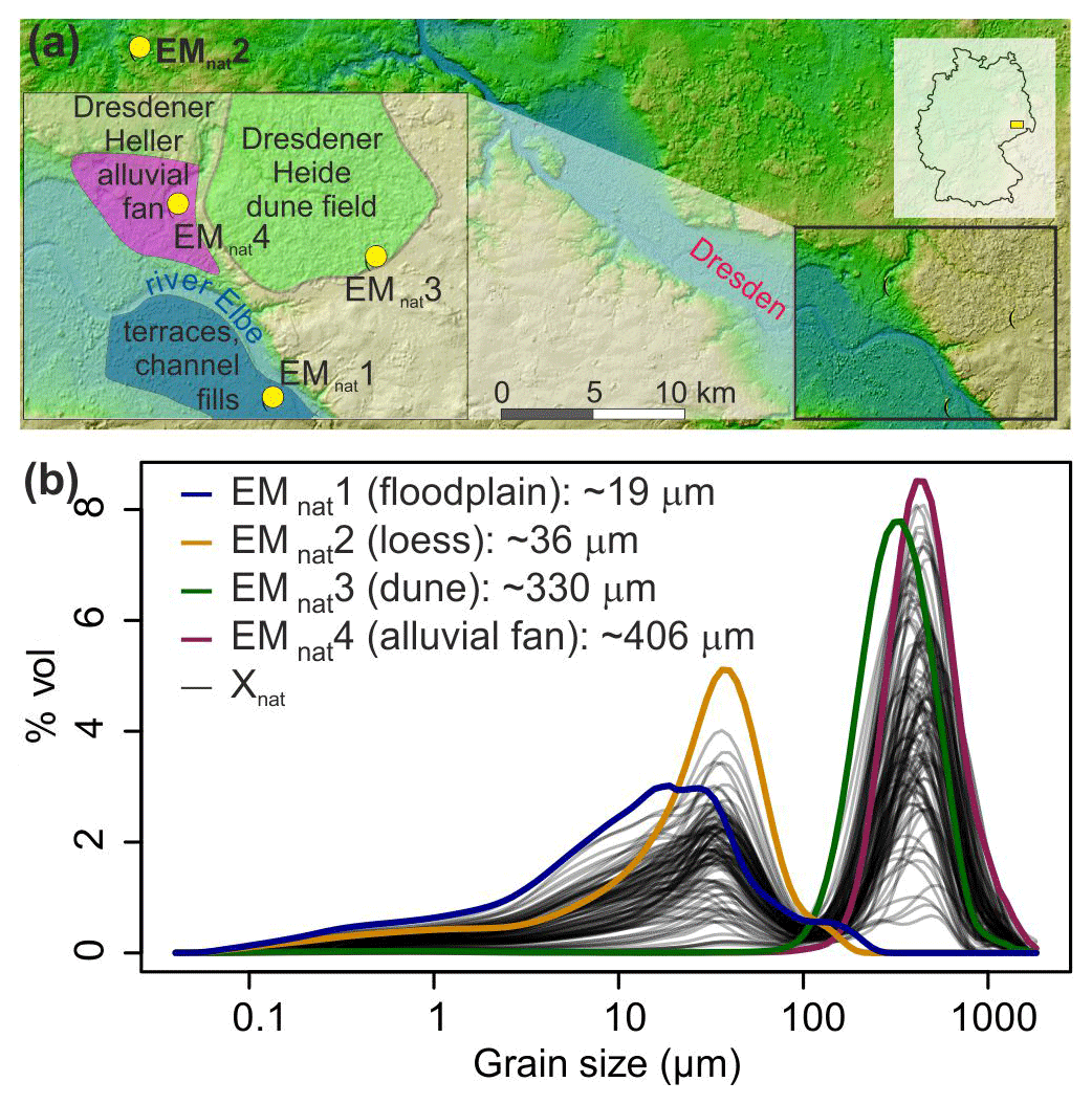
Figure 2 (a) Sample locations and sedimentological setting (according to the geological map, section Dresden, Sächsisches Landesamt für Umwelt, Landwirtschaft und Geologie; http://www.geologie.sachsen.de/geologische-karten-14041.html, last access: 10 May 2019); see kmz file in the Supplement. (b) Grain-size distributions of the four natural grain-size end-members (EM_nat) and the 100 resulting mixed samples (X_nat), i.e. the example data set of the EMMAgeo R package (Dietze and Dietze, 2019).

Three parallel samples (0.3–2.0 g) per outcrop were chemically treated with 10 % NaCl, 15 % H₂O₂ and 1.25 mL Na₄P₂O₇, each for 48 h, and measured with a Beckman Coulter LS 13 320 Laser Diffraction Particle Size Analyzer at RWTH Aachen, delivering 116 classes (0.04–2000 µm). Between 7 and 16 aliquots per sample were investigated in triplicates. Grain-size distributions were derived applying the Mie theory with the following parameters: fluid refraction index: 1.33; sample refraction index: 1.55; imaginary refraction index: 0.1. The resulting median grain-size distributions (Fig. 2) were manually mixed in the lab to generate 100 samples with randomly assigned individual contributions. Within this data set X_nat, 50 samples contained all four EM_nat, 25 were prepared without EM_nat4 material and a further 25 were prepared without EM_nat1. Hence, in contrast to other studies, we fully know the grain-size distributions of the underlying natural process end-members and their mixing ratios, which allows a detailed evaluation of performance and comparison of all available EMMA algorithms.

3.2 Model performance of different EM analyses

The example data set X_nat was decomposed with deterministic EMMA of EMMAgeo using q=4 and l=0. Robust EMMA was run with both the extended and the compact protocol. To be as conservative and as unbiased as possible, both protocols were executed with the default parameterisations as suggested above and were only modified when results obviously prompted manual parameter adjustments.

To run the FORTRAN-based approach by Weltje (1997), provided by Jan-Berendt Stuut (personal communication, 2017), the grain-size classes of X_nat needed to be aggregated; i.e. the resolution decreased by a factor of 2. For consistent comparisons with the other approaches, the resulting end-member loadings were interpolated back to the initial grain-size resolutions (see Supplement). The down-sampling and subsequent up-sampling of all EM_nat values resulted in negligible artefacts with an average R²>0.999. The modelled data set X^′ was computed by combining loadings and scores according to Eq. (1), excluding the error matrix E.

Running the collection of the five RECA R scripts (Seidel and Hlawitschka, 2015) required manual installation of the additional package compositions (Van den Boogaart et al., 2014), e1071 (Meyer et al., 2017) and nnls (Mullen and van Stokkum, 2012), loading all scripts and manual screen input of the model parameters. RECA needs to be run completely to the end until consequences of parameter changes can be inspected. The decision on q is based on a q–$R_n^{\mathrm{2}}$ plot (e.g. using the inflection point). Here, RECA was run with four end-members, a maximum convexity error of −6, confirmation of the first start model, 100 iterations and a weighting exponent of 1, as suggested by Seidel and Hlawitschka (2015).

AnalySize by Paterson and Heslop (2015) provides a MATLAB GUI, in which q is set manually. The numeric MATLAB output, end-member loadings and scores, was imported to R using the package R.matlab (Bengtsson, 2018).

Bayesian EMMA (BEMMA) in MATLAB (Yu et al., 2015) does not allow a predefined q to be specified. With repeated model runs, the number of output end-members changed unsystematically between two and four. Depending on q, the shape and mode positions of the unmixed distributions fluctuated, which prevented the output from different model runs from being grouped. Hence, we did not include BEMMA in this comparison.

3.3 Evaluation and validation criteria

The performance of all approaches was evaluated in two steps. First, we compared the original data set X_nat and the modelled data sets X^′ using (i) coefficients of determination (mean total $R_{\mathrm{t}}^{\mathrm{2}}$, sample-wise $R_m^{\mathrm{2}}$, class-wise $R_n^{\mathrm{2}}$) and (ii) the absolute differences between X_nat and X^′ (total MAD_t, sample-wise MAD_m, class-wise MAD_n). This comparison resembles the classical evaluation step when the true natural end-member composition is unknown.

Second, knowing which natural end-members have been mixed to create the example data set X_nat, we compare (i) R² and MAD for EM_nat distributions and loadings ($R_{n\mathrm{1}}^{\mathrm{2}}$ to $R_{n\mathrm{4}}^{\mathrm{2}}$ and MAD_n1 to MAD_n4), (ii) R² and MAD for mixing ratios and scores ($R_{m\mathrm{1}}^{\mathrm{2}}$ to $R_{m\mathrm{4}}^{\mathrm{2}}$ and MAD_m1 to MAD_m4) and (iii) the absolute deviations of the mode positions of EM_nat distributions and loadings. For comparisons of EM_nat distributions with modelled loadings, all results were truncated to grain-size classes of EM_nat higher than 0.1 % vol and rescaled to 100 %. There are two reasons for this: first, due to the generally narrow grain-size distributions, EM_nat contained many grain-size classes of only zeros, which biases the resulting measures (Ciemer et al., 2018). This bias is severe: correlating, for example, two sequences of random values (e.g. 3.1, 5.2, 4.0 and 9.2, 8.3, 3.5) typically yields a very low correlation coefficient (e.g. $r=-\mathrm{0.065}$). However, padding these sequences with zeros strongly increases the correlation coefficient (e.g. r=0.87, including five zeros). Second, it is known that EMMA (Dietze et al., 2012), but also other approaches, causes spurious secondary modes directly below the mode positions of other end-members (Paterson and Heslop, 2015). The spurious modes are obviously not related to the underlying sedimentation regime and are not intended to be interpreted genetically (Dietze et al., 2014). As they would also bias the model comparison measures, we excluded them from model evaluation.

4 Results: the different model performances

4.1 Evaluation of model performance

4.1.1 Deterministic EMMA

Figure 3 shows the default graphical output after the EMMA algorithm has modelled the data set with four end-members. Panels a and b depict R² values (squared Pearson correlation coefficients) organised by grain-size class and sample. Overall, the data set was reproduced with a mean $R_{\mathrm{t}}^{\mathrm{2}}$ of 0.969 and MAD_t of 0.2 % vol (Table 1). Panels c and d show modelled end-member loadings and scores. End-member loadings (EM1-4) had modes at 16, 40, 310 and 450 µm. Spurious secondary modes of less than 2.5 % vol are visible below primary modes of other end-members. Apart from the multi-modal EM4, all end-members have a log-normal shape. Figure 3a shows that grain-size class-wise $R_n^{\mathrm{2}}$ decreases between 946 and 1830 and 117 and 177 µm, both grain-size class intervals that contribute less than 0.9 % vol to X (Fig. 2). Mean sample- and class-wise absolute deviations are shown in Table 1.

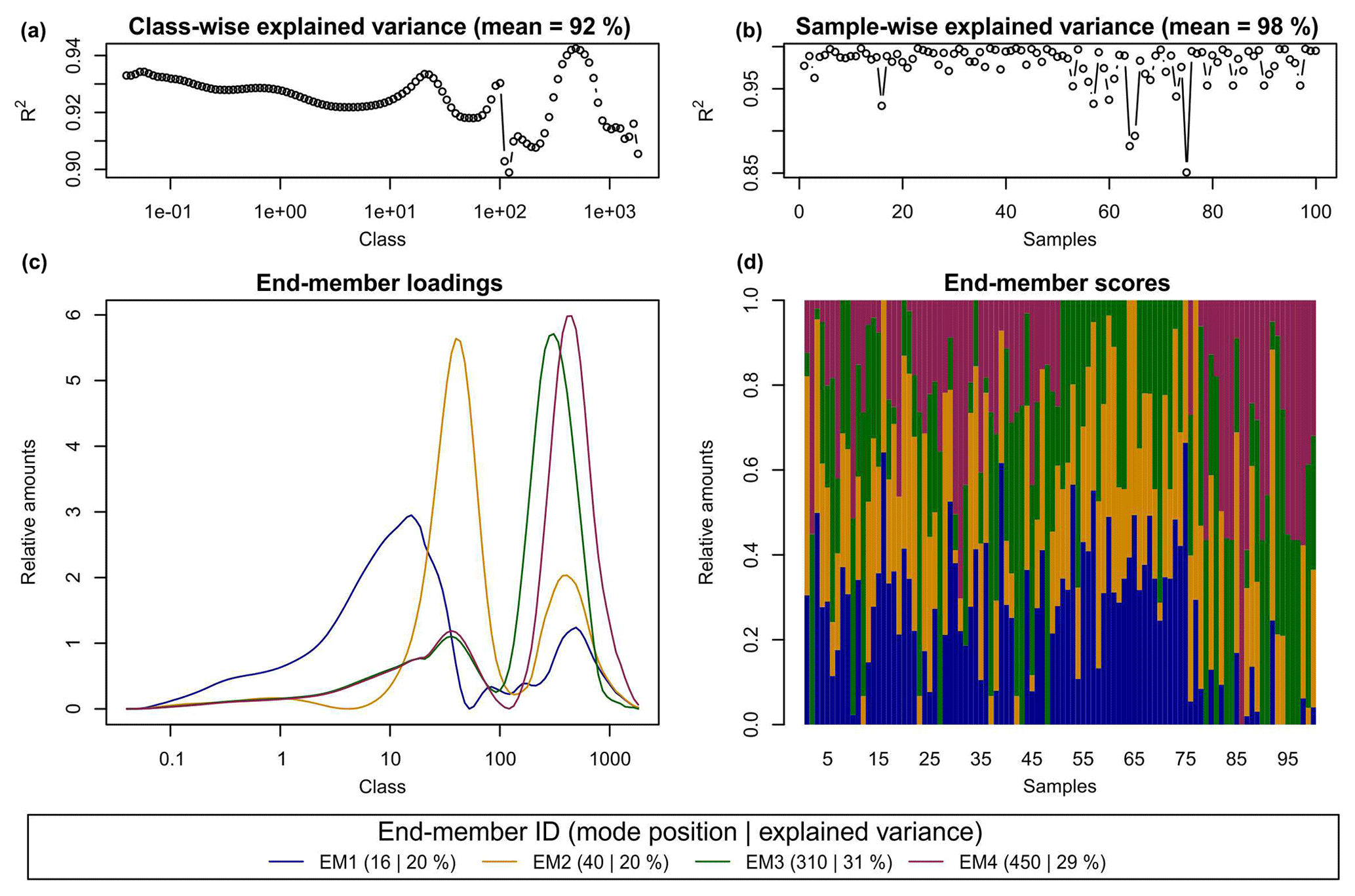
Figure 3 Default graphical output of the R function EMMA(). (a, b) Measures of model performance (i.e. class- and sample-wise R²), (c) end-member loadings and (d) end-member scores. The legend presents the main mode positions (µm) and explained variance of each end-member (%).

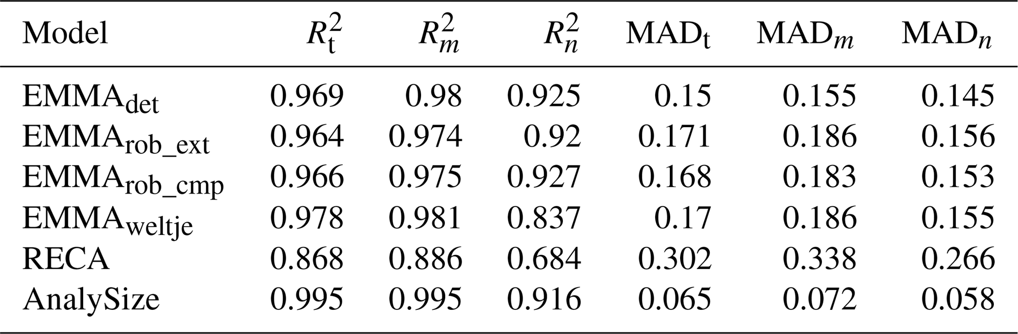
Table 1 Comparison of model performance (total, sample-wise and grain-size class-wise coefficients of variation ($R_{\mathrm{t}}^{\mathrm{2}}$, $R_m^{\mathrm{2}}$, $R_n^{\mathrm{2}}$) and absolute deviation (MAD_t, MAD_m, MAD_n) of X_nat versus X^′). EMMA_det, EMMA_{rob_ext} and EMMA_{rob_cmp} refer to EMMAgeo deterministic, extended and compact robust models (see text). EMMA_weltje, RECA and AnalySize refer to end-member approaches in FORTRAN (Weltje, 1997), R (Seidel and Hlawitschka, 2015) and MATLAB (Paterson and Heslop, 2015), respectively.

The scores of EM1 to EM4 accounted for 20 %, 20 %, 31 % and 29 % of the variance of X^′, respectively. Sample-wise $R_m^{\mathrm{2}}$ is 0.98 on average (Table 1). Four outliers had $R_m^{\mathrm{2}}<\mathrm{0.95}$ (samples 16, 57, 64, 75; Fig. 3b). However, neither removing these samples nor changing the rotation type from Varimax to Quartimax or the oblique rotation Promax improved the modelling of loadings and scores (not shown).

4.1.2 Robust EMMA – extended and compact protocol

In the extended protocol, an l_min of zero was used according to Miesch (1976), and l_max was set to 0.37, i.e. 95 % of the modelled absolute l_max of 0.39 (see methods in Sect. 3). However, when using this value, negative loadings occurred. Therefore, the value was set to 80 %, yielding a more realistic and valid l_max of 0.31. With 20 values between l_min and l_max, q_min varied between 2 and 3 (Fig. 4a), and q_max showed a trend of decreasing ${\mathit{R}}_{\mathrm{t}}^{\mathrm{2}}$ with increasing l (Fig. 4c, d), until even NA values were produced for some parameter combinations (blue graph, Fig. 4b). Accordingly, after a local optimum at q_max between 4 and 9 (open circles, Fig. 4b), adding more end-members leads to numerical instabilities.

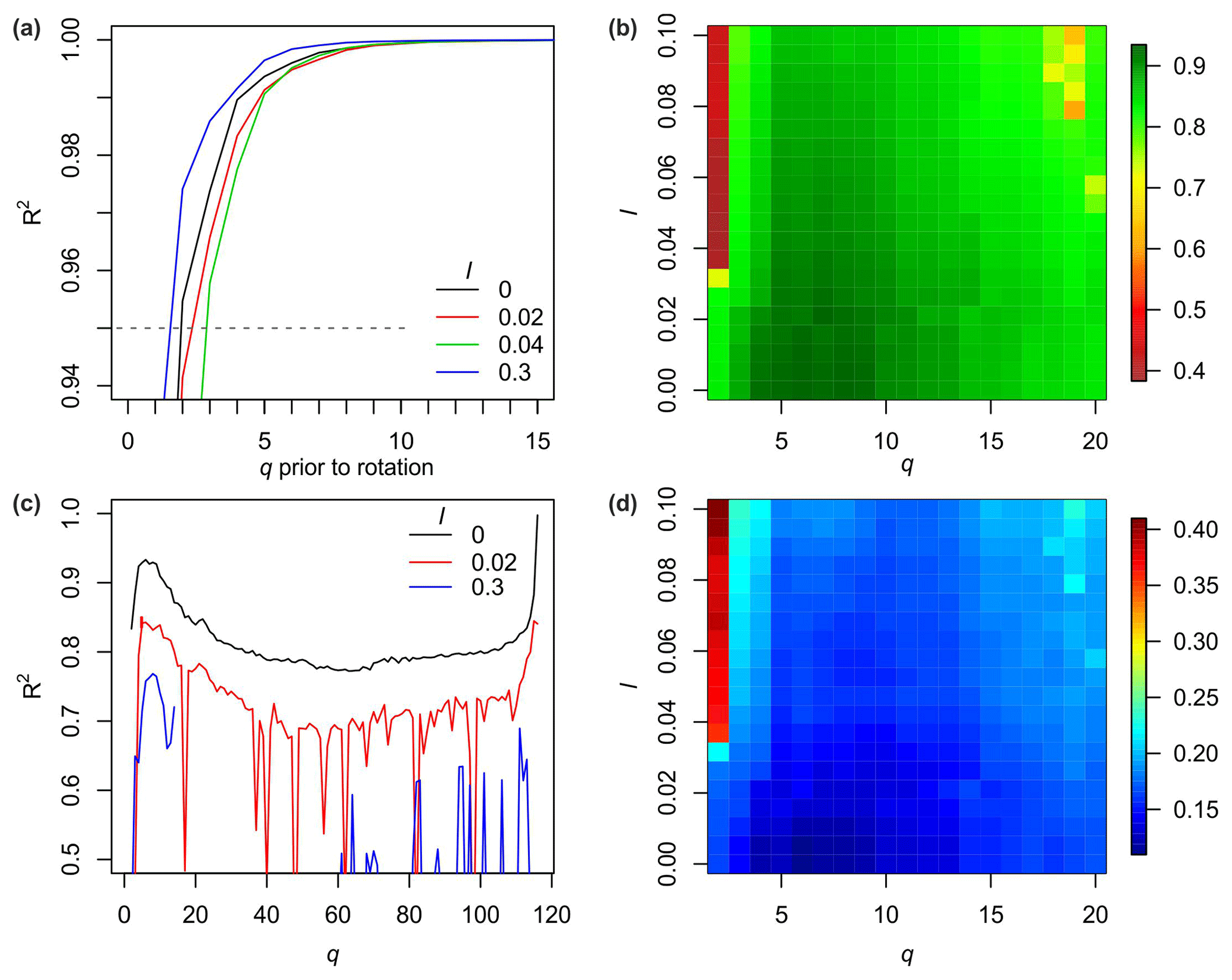
Figure 4 Parameter optimisation steps in the extended protocol of robust EMMA. (a) Model performance (coefficient of determination) with increasing number of factors prior to rotation (examples of weight transformation limits l; default output of the function test.factors()). (b) Mean total $R_{\mathrm{t}}^{\mathrm{2}}$ of all likely q and l, default output of test.parameter(), 19 different q (2 to 20). (c) Examples of total $R_{\mathrm{t}}^{\mathrm{2}}$ of EMMA-scenarios as a function of the number of end-members q (along the x axis) and three different l values. (d) Mean sample-wise model error E_n of all likely q and l values, optional output of test.parameters(), 20 different l values (0 to 0.1).

Figure 5a shows all 223 end-member loadings from 96 EMMA runs that agree with the parameter space of P. Note that the protocol can be run with user-defined grain-size units (function argument classunits) or simply the raw grain-size class numbers (default, and used in the following sections for simplicity). Several end-members have main mode position clusters between grain-size class numbers 63 and 66, 74 and 77, 94 and 97 and 99 and 102 (orange polygons). These class limits were used to model the robust end-member loadings, excluding the negative loadings that were modelled due to l_max values that are too high. A fifth cluster at classes 71–73 exists (not marked), although the distribution of this end-member is rather broad and overlaps with the distribution shapes of the two other clusters in this range. It was rejected as a robust end-member (see below).

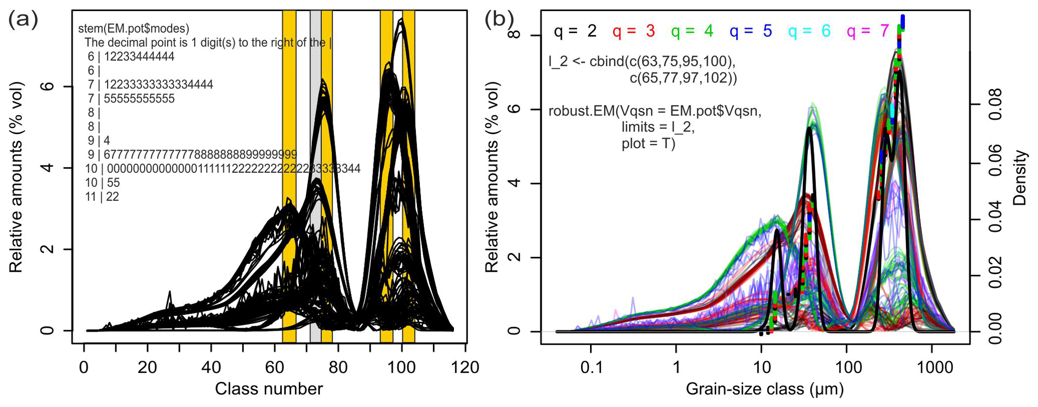
Figure 5 (a) Potential end-member loadings resulting from multiple EMMA runs with similarly likely parameter combinations. Distinct clusters of main mode positions define the grain-size class limits (orange bars) and allow calculation of the range of robust end-members by averaging the loadings with main modes that fall within the defined class limits. Note that there is no straightforward impression of the four input EM_nat values and the few, spikey loadings resulting from values of l that are too high. A stem-and-leaf plot of the mode clusters can be used to judge the appropriateness of the identified limits. (b) Default graphical output of the R function model.EM() assigns potential end-member loadings to the EMMA runs of (a). Coloured lines show end-member loadings from EMMA models with different q (dots at respective main mode positions) and varying l values. The black line is a kernel density estimate of the main mode positions of all loadings, with a default bandwidth of 1.16, i.e. 1 % of the number of grain-size classes of the input data set and a default threshold to identify mode clusters (i.e. 0.016) that define three robust end-members (not shown). Manual setting of the limits avoids overlapping of the two coarse end-members and excludes the loadings of the grey bar.

The resulting robust EM3 and EM4 loadings show high class-wise standard deviations (SDs) around the mode positions (Fig. 6a). EM1 has a continuously narrow uncertainty envelope (i.e. mean±1 SD), and EM2 shows the largest and most variable envelope. Mean class-wise SDs range from 0.06 (EM4) to 0.38 % vol (EM2). The main mode positions of the robust loadings are identical with those of deterministic EMMA; only the EM2 mode is one class off. Using the mean robust loadings, l_opt was 0.0163 when maximising $R_{\mathrm{t}}^{\mathrm{2}}$. Based on this, mean robust scores were modelled (Fig. 6b) with an average SD of 9.9 % vol, 7.8 % vol, 11.3 % vol and 9.5 % vol for EM1 to EM4.

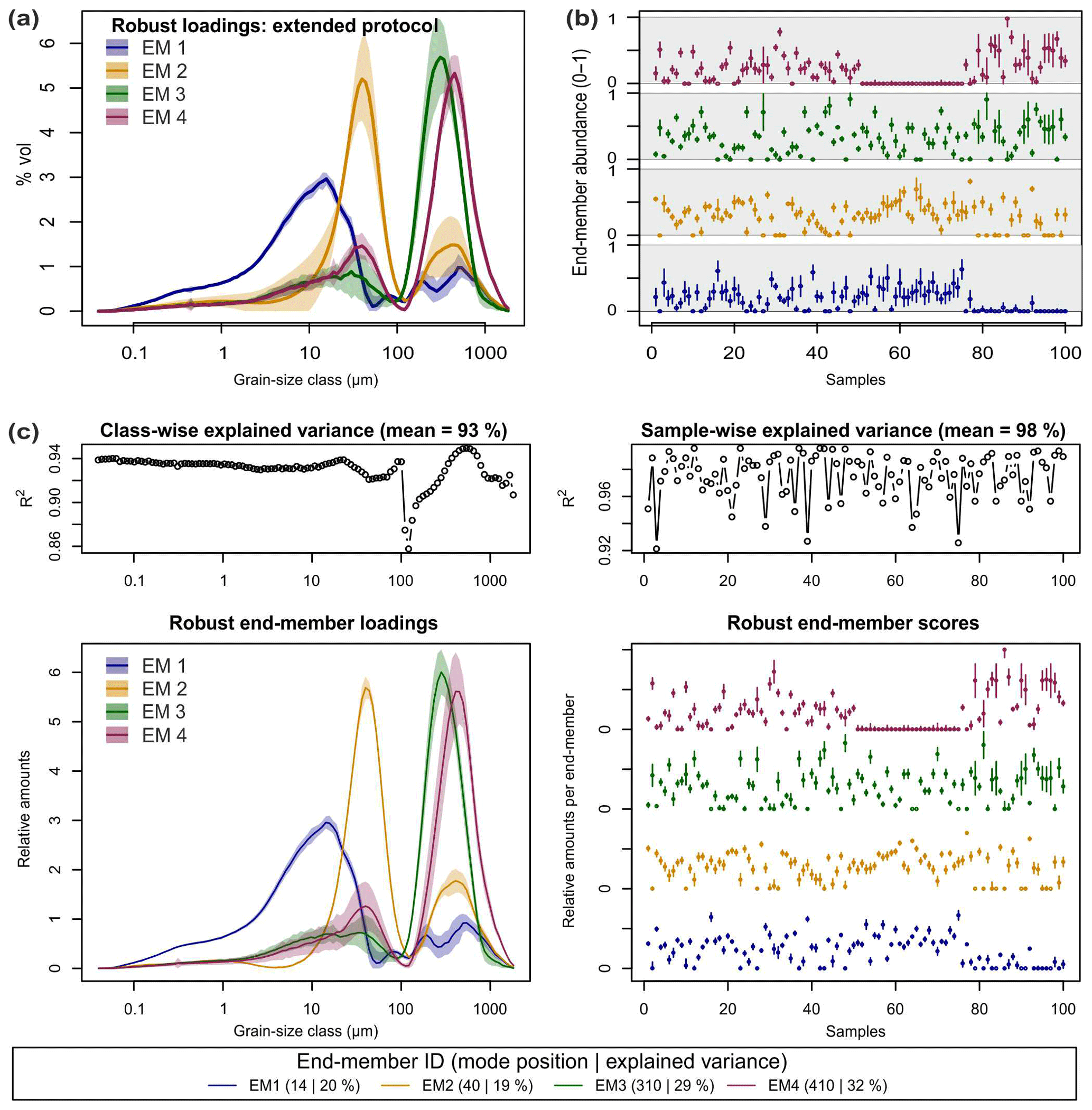
Figure 6 (a) Robust end-member loadings and (b) scores of the extended protocol. (c) Default graphical output of robust.EM() as part of the compact protocol, including class- and sample-wise explained variances (a, b) and a legend with main mode position and explained variance of each end-member. Mean robust loadings as line graphs, mean robust scores as panels of points. Polygons around loadings and bars around scores represent 1 standard deviation.

With the compact protocol, the same parameter space (l_min, l_max, q_min and q_max) was calculated as with the extended protocol. Robust end-member definition is supported by the plot output of the function robust.EM(). Figure 5b shows five clusters with mode positions at 13–16, 27–33, 38–47, 250–320 and 390–500 µm (i.e. class numbers 63–66, 71–74, 75–77, 95–97 and 100–102). The colour scheme reveals that the cluster at 27–33 µm (grey bar, Fig. 5b) systematically occurs when EMMA was run with three end-members (red curves, Fig. 5a). Clusters at 13–20 and 38–47 µm emerge especially when four end-members were included in a model run (green curves). A similar case exists for the two coarse end-members, at 250–320 and 390–500 µm. Hence, models with a value for q that is too small systematically merge distinct grain-size distributions into spurious, broad curves. Values for q that are too high instead caused spikey loadings (blueish, pink curves, Fig. 5b).

Defining the limits by the automatic kernel density estimate approach suggested only three out of four natural end-members as robust ones, combining all loadings around class 100 (Fig. 5b, black line). Setting the kernel bandwidth arbitrarily to 0.5 would allow separation of the two overlapping modes around EM_nat2 while missing EM_nat1 and misinterpreting the cluster around the two coarsest end-members (not shown). Thus, for strongly overlapping mode clusters, automatic class limit detection was not appropriate. Hence, we set the mode limits similar to the extended protocol to class numbers 63–66, 75–77, 94–97 and 99–102, changing the definition of EM2 by just one grain-size class (extended protocol: 74–77) to better exclude the cluster at 27–33 µm (red curves, Fig. 5b) and to assess varying robust end-member definitions.

The resulting end-members are shown in Fig. 6b. They are similar to the plotted output of the deterministic version (Fig. 3) but extended by uncertainty polygons, the different representation of scores and slightly different mode positions, grain-size class-wise $R_n^{\mathrm{2}}$ (0.93) and sample-wise $R_m^{\mathrm{2}}$ (0.98). Mean end-member contributions to the variance of the data set (20 %, 19 %, 29 % and 32 %) are almost identical to the deterministic version.

4.1.3 Comparison to other end-member unmixing algorithms

The full benchmark reveals that all approaches successfully model the data sets. The output of RECA shows difficulties in reaching the minimum convexity error of −6 with the initial 100 iterations, but by increasing the value to 200 iterations the issue was solved.

The average $R_{\mathrm{t}}^{\mathrm{2}}$ values were higher than 0.868 in all cases, up to 0.995 (Table 1). Sample-wise $R_m^{\mathrm{2}}$ values were always higher than the grain-size class-wise $R_n^{\mathrm{2}}$ values. Deterministic EMMA yielded slightly better results than the two robust EMMA protocols, which in turn were very similar. The lowest (highest) and highest (lowest) $R_{\mathrm{t}}^{\mathrm{2}}$ (MAD_t) values are related to RECA and AnalySize, respectively.

The main absolute deviations of X^′ from X_nat are associated with grain-size classes between 100 and 1000 µm, regardless of the model (Fig. 7). Except for AnalySize, all approaches show systematic underestimation of these grain-size classes of up to −2.5 % vol per class. Vice versa, finer grain-size classes between 1 and 100 µm are slightly overestimated by ca. 1 % vol per class. The effects of the applied sample mixing scheme of X_nat are clearly visible in all model results (Fig. 7). Samples 51 to 75 (without coarse EM_nat4) show an overestimation of coarse and underestimation of fine classes. Samples 76 to 100 (without fine EM_nat1) show the opposite picture. AnalySize yielded the overall best unmixing, with average deviations of ca. ±1 % vol.

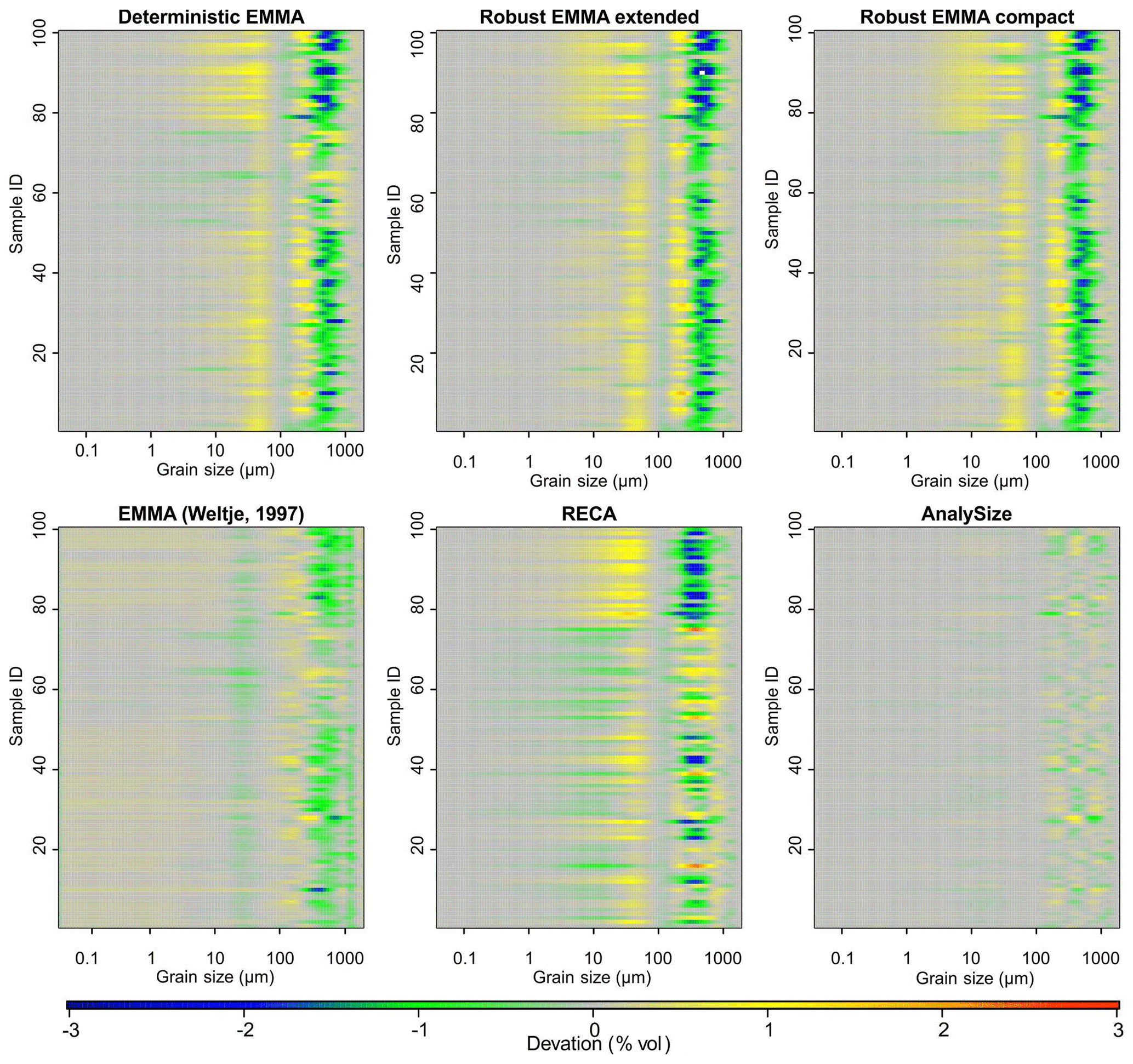
Figure 7 Model performance to unmix and reproduce the example data set X_nat. For each end-member model approach, the absolute difference MAD between modelled and original data set is shown.

4.2 Validation against known data set composition

The above criteria quantify how well the approaches modelled the data set (Eq. 1), whereas their ability to reproduce the true “mixed ingredients” is addressed here. The R² values between loadings and input EM_nat grain-size distributions (Table 2a) were on average between 0.4 and 0.99 and, thus, systematically larger than R² values linking scores and mixing ratios (0.77 to >0.99; Table 2b). Both EMMAgeo and AnalySize performed less well in modelling one out of three EM_nat distributions (EM1 for EMMAgeo and EM4 for AnalySize). The MAD was below 0.8 % vol for all models and end-members, except for EM4 scores (AnalySize).

Table 2 (a) Grain size class-wise coefficients of variation ($R_n^{\mathrm{2}}$) and absolute deviation (MAD_n) of modelled end-member loadings compared to natural end-member distributions. (b) Sample-wise coefficients of variation ($R_m^{\mathrm{2}}$) and absolute deviation (MAD_m) of modelled end-member scores compared to natural end-member mixing ratios.

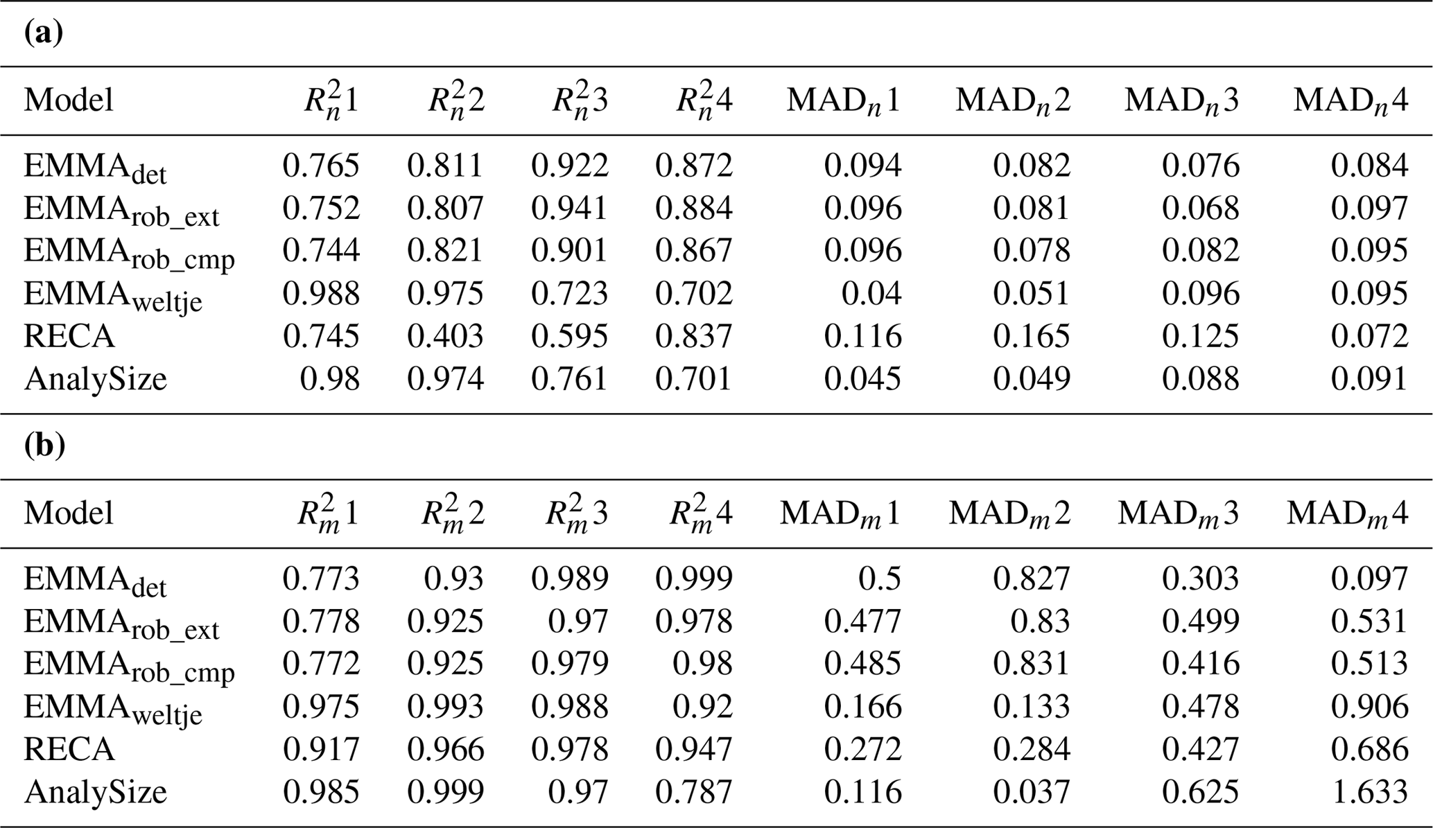
A graphical comparison of the grain-size class-wise deviations of input end-member distributions and modelled loadings (Fig. 8) shows that all EMMAgeo-based models underestimate the main mode grain-size classes (i.e. curves are below the 1:1 line). This is the result of the emergence of spurious modes that shift class-wise percentages (up to −3.2 % vol) from the main modes to classes around the spurious modes (up to 1.3 % vol) that actually contain no grains (vertically aligned points at zero x values). The other EMMA approaches also show mismatches between natural end-members and modelled loadings. Especially the alluvial fan EM_nat4 is affected, most severely in AnalySize. Percent volume (% vol) shifts due to spurious secondary modes also occur for the algorithm of Weltje (1997) and RECA. Overall, the latter approach yields the most accurate representations of the input distributions.

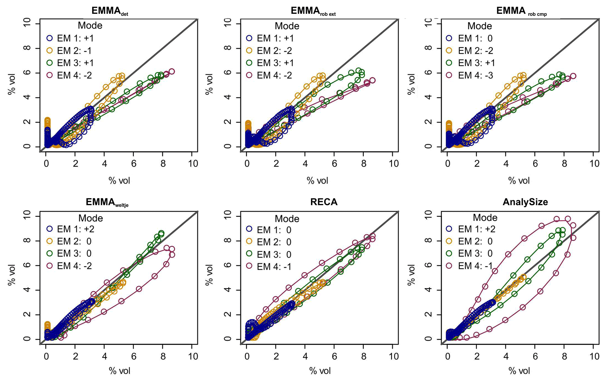
Figure 8 Natural versus modelled end-member grain-size distributions for all evaluated models. Deviation of main mode (in number of classes). x axes show X_nat and y axes modelled X^′ values.

Concerning the reproduction of the initial mixing ratios (Fig. 9, Table 2b), variability among the models is higher, and all approaches show some unsystematic over- and underestimation, especially for EM in samples in which real mixing ratios were zero (vertical point clusters along the 0 % x axis; Fig. 9). Except for RECA and AnalySize, the opposite effect is also visible: the models suggest zero contribution from end-members that are actually present in a sample with up to ca. 20 % (horizontal points along the 0 % y axis; Fig. 9).

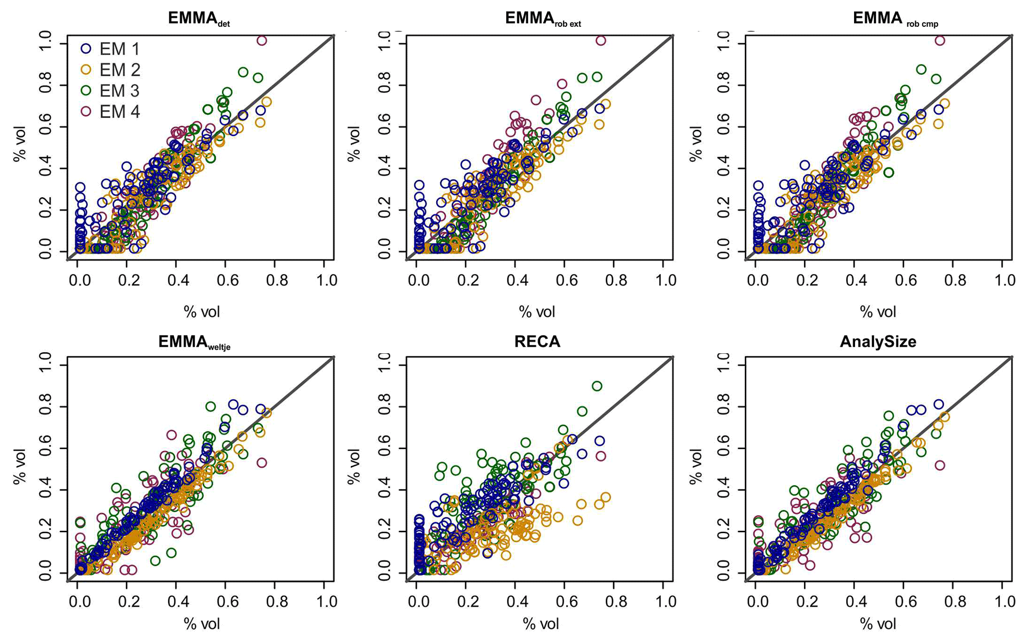
Figure 9 Natural versus modelled end-member mixing ratios for all evaluated models. x axes show X_nat and y axes modelled X^′ values.

The modal grain-size classes of the four EM_nat were modelled with different levels of success (Fig. 8, legends). The main modes of the coarse end-members were detected with only one or two grain-size classes' difference, whereas finer end-members differed by up to three classes. Modal classes of EM_nat2 and EM_nat3 were correctly depicted by EMMA of Weltje (1997), RECA and AnalySize. Most models yielded a value of EM_nat1 that is slightly too coarse, deviating by one or two grain-size classes. EM_nat4 caused the largest scatter among the models.

5 Discussion

5.1 Operational modes of EMMAgeo

The functionality of EMMA has improved significantly since the introduction of the MATLAB algorithm of Dietze et al. (2012). Not only an increase in computation speed, which was already 1 to 3 orders of magnitude faster than for other algorithms (Paterson and Heslop, 2015), but also many new and detailed ways to explore end-members (with deterministic EMMA) and to estimate and describe associated uncertainties of all end-member components (with robust EMMA) were implemented. The plot output of both EMMA modes is a comprehensive visualisation of all relevant information. It allows direct process interpretation in terms of plausibility of loadings and scores, model performance and identification of outliers.

Both EMMA modes, deterministic and robust, result in consistently similar outputs. Deviations of individual modes of robust loadings from known EM_nat distributions by one or two grain-size classes are within the model uncertainty of robust EMMA. Therefore, a key step is the definition of robust end-members by setting the grain-size class limits that bracket robust, parameter-independent main modes, which overcomes the problem of relying on statistical measures like the inflection point of a q–R² graph (van Hateren et al., 2018). The workflow of robust EMMA offers ways to explore the ability of different kernel bandwidths and density thresholds, but in complicated cases, like the one provided in this study, expert knowledge-based limit definition might be the most practicable option. Hence, each data set should be considered individually, and deviations from common patterns may be significant in their own right (see discussion by van Hateren et al., 2018).

5.2 Performance test and validation

Unmixing quality is very high regardless of the model used, suggesting that all approaches in this benchmark are able to reproduce the input grain-size data set with unmixed end-member subpopulations. There is no model with an outstanding performance. Model deviations of <1 % (especially for grain-size classes with >0.1 % vol) are low in the light of uncertainties related to process interpretation (see below).

The validation against known input end-member composition showed that all EMMA approaches are equally applicable. When comparing end-member loadings with the EM_nat distributions, R² mainly represents shifts in mode positions, whereas MAD reacts to both shifts in the modes of individual grain-size distributions and differences in the volume percentages per class. Yet, each algorithm has certain strengths depending on the specific dimension of the investigation: if the main goal is to identify the most likely q that builds an empirical data set, robust EMMA provides a set of tools that go beyond classical approaches (e.g. the inflection point of the q–R² plot) – allowing the inclusion of expert knowledge in the quantification and interpretation of grain-size subpopulations.

If the correct grain-size distribution shape of underlying process end-members is targeted, RECA of Seidel and Hlawitschka (2015) and EMMA by Weltje (1997) are most suitable from our benchmark study (Table 2a). RECA had problems with reaching the convexity error threshold, which could result from our data set with largely overlapping natural process end-members.

When quantifying the contribution of end-members to a given sample, robust EMMA, EMMA according to Weltje (1997) and AnalySize performed best (Table 2b). Robustly estimated scores using EMMAgeo reproduced original mixing proportions very well and in a range comparable to the other available end-member algorithms. However, as all approaches and earlier EMMA evaluations showed, very low and high scores (<20 % and >80 %) of one end-member might be under- or overestimated within the compositional mixture (McGee et al., 2013). Hence, extremely high (e.g. 100 %) contributions of one end-member to a sample should not be interpreted as complete absence of the other end-members but rather as the dominance of this one end-member (and vice versa).

If uncertainty estimates for both loadings and scores are considered important, then only robust EMMA is suitable. The inclusion of uncertainties for loadings and scores is a key precondition for propagating model results to further data analysis, for example to interpret grain-size end-members as proxies for sediment sources (loadings) in environmental archives as they evolve with time (scores). As van Hateren et al. (2018) emphasise, changes in the model results will inevitably result in diverging interpretations of the assumed sedimentary processes. Also, the interpretations of the scores in their spatial (samples across a landscape) or temporal (samples downcore) context will be affected. Thus, it is extremely important to provide some estimate of the inherent uncertainty in both the proxy definition and in the sample domain. So far only robust EMMA can deliver such information. Yet, necessary parameter estimates and diverging start conditions evidently exist in the other models too.

If the distribution shape of an inherent natural grain-size end-member is known, EMMAgeo allows quantification of its contribution to the data set by including it as unscaled loadings in both deterministic and robust EMMA or by assigning the known main mode class limits when selecting robust end-members (step 4; Fig. 1b). Finally, if free and open-source software is a criterion – which is increasingly the case for journals and funding agencies (David et al., 2016; Munafò et al., 2017) – RECA and EMMAgeo remain the only options.

5.3 Comparison with other benchmark studies

In previous benchmark studies, EMMAgeo performed less well, which Paterson and Heslop (2015) attributed to the implementation of the non-negativity and sum-to-one constraints. van Hateren et al. (2018) pointed to the secondary modes as cause of the deviations of scores from the mixing ratios. We cannot confirm the poor performance of EMMAgeo in our study, as it is not fully clear how van Hateren et al. (2018) determined the EMMAgeo loading curves, which they evaluate graphically. They note that in EMMAgeo the q is not set by the inflection point of the q–R² relationship, but robust EMMA would lead to one q, and not a sequence of 2 to 5, as discussed in their study. Additionally, it is unclear which realisation from within the robust EMMA uncertainty range was evaluated by van Hateren et al. (2018). Accordingly, detailed introduction of the EMMA protocols is essential to avoid future misinterpretations.

Yet, the occurrence of artificial secondary modes below the main modes of the end-members is more pronounced in EMMAgeo compared to other unmixing algorithms. The inherent compositional data constraints lead to an intimate linkage of the distribution shape of one end-member with the distribution shapes of other loadings. However, when excluding hardly interpretable secondary modes from global measures of model quality, the performance of EMMA is well within the range of other available algorithms. As repeatedly noted in articles applying EMMAgeo (Dietze et al., 2012, 2014) but also highlighted for other approaches in the benchmark study of Paterson and Heslop (2015), secondary modes are model artefacts and should not be interpreted genetically.

However, to test the impact of artificial secondary modes on model performance, we modelled the EM_nat data set with user-defined end-members. We manually set the unscaled loadings outside the known primary end-member modes to zero and used these updated loadings for the modelling process (see Supplement for R code). Although the resulting end-member loadings are now free of secondary modes, the mixing ratios are only marginally better modelled (−1 % to 4 % deviation). Thus, such a truncation may help in tuning the shape of the modelled end-members but cannot improve deviations of the scores from mixing ratios. Still, the uncertainty ranges of the robust scores included the expected EM_nat mixing ratios (66.5 % of the samples are within the modelled 1 standard deviation range).

5.4 Constraints on end-member interpretation

Going beyond classical measures of grain-size properties, EMMA is well suited to quantify sedimentary processes from mixed sediment sequences in space and time. However, interpretation of grain-size end-members requires expert knowledge about the investigated sedimentary system. Hence, when applying EMMA to any set of grain-size data, the interpretability of the resulting end-members needs to be checked. For this, both end-member components should be considered: the shape and position of the main modes of the loadings and the spatio-temporal or stratigraphic context of the scores. For example, the effectiveness of a process in sorting sediment could be interpreted in the classical sense from the shape of the end-member loadings (excluding artificial modes), with broader peaks being more poorly sorted than narrow peaks (Friedman, 1961).

As any other statistical method, EMMA is a tool, and interpretation of grain-size end-members relies on contextual knowledge. There may be processes that contribute to the overall sediment composition and that are not size-selective or sort sediment of various grain-size classes in a typical way. For example, event-triggered turbidity currents in lakes caused problems in attributing a single sedimentary process to end-members in the study by Dietze et al. (2014) because the typical fining-upwards trend was also reflected by several end-members that contributed to samples of “normal” deposition.

Closely related is the constraint of stationarity in processes, which implies that through space and time each transport process must create an identical grain-size distribution. For example, fining of aeolian material from one distinct source area with downwind transport distance (Pye, 1995) might rather be explored by a gradual approach, e.g. by running EMMA in a moving window over a data set to detect shifts in stationarity.

Post-depositional processes that change grain-sizes, e.g. due to permafrost conditions or soil formation, could strongly disturb the original grain-size characteristics. In the worst case, a lacustrine sediment archive composed of different aeolian and fluvial sediment end-members (Dietze et al., 2013) can be affected by ongoing cryogenic and active-layer dynamics in a way that all modelled end-members were overlapping and peaking in similar grain-size classes – “erasing” primary signals related to sediment deposition. If post-depositional activity overprints the original depositional processes, EMMA can detect them as single end-members and would allow quantification of the intensity of the overprint, e.g. soil formation (Dietze et al., 2016) or weathering (Sun et al., 2002; Xiao et al., 2012).

Sediments affected by the processes mentioned above can affect end-member modelling in manifold ways. For example, EMMA could result in rather low explained variances, and the modes of affected end-member loadings would become broader and/or may even be better represented by additional but nevertheless spurious end-members. In the worst case, modes of end-member loadings overlap strongly or cannot be unmixed at all.

6 Conclusions

EMMAgeo allows the characterisation of multi-modal grain-size distributions by end-member subpopulations. New protocols allow a quick analysis, including modelling of associated uncertainties for both end-member loadings and scores. Using four known natural end-members, which represent typical sediment types found in terrestrial systems, the performance of EMMAgeo in unmixing the correct end-member distribution shapes and mixing ratios is within the same order as the performance of other available end-member modelling algorithms, which all perform very well. Hence, all of these algorithms are powerful tools for characterisation of different sediment source, transport, depositional and even post-depositional processes. In comparison to other algorithms, EMMAgeo is the only available open-source grain-size unmixing approach that includes uncertainty estimates. An inherent strength of the fully free R package is a large flexibility for users to modify the parameter settings and workflows with the new protocols, reproduce results and continue data evaluation.

Once genetically interpretable grain-size end-members are derived, their loadings can be described by classical descriptive measures (Folk and Ward, 1957; Blott and Pye, 2001). This allows a statistically robust determination and comparison of mean, sorting and shape measures across sites and data sets by describing and quantifying processes that sort sediment better or poorer than other processes.

Many future applications in the fields of Quaternary Science, sedimentology, geology, geomorphology and hydrology could gain new insights from applying EMMAgeo to compositional data sets that represent mixtures. In contrast to classical linear decomposition methods such as principle component analysis, EMMA has the potential to quantify (and not just qualify) different sources or processes of modern and past sedimentary environments that contribute to a sample set, including associated model uncertainties.