Sediment storage quantification in the Black Forest highlights tectonic influence on typically wide and shallow valleys

Quantifying sedimentary volumes in mountain valleys can not only enhance our understanding of Quaternary valley evolution and river dynamics but also yield critical insights into hydrogeological characteristics. In contrast to the thoroughly investigated Upper Rhine Graben, little coherent information is available on the subsurface structure of adjacent Black Forest valleys. This study therefore aims at estimating the thickness, spatial distribution, and volumes of alluvial material in the valleys of the southwestern Black Forest. We utilized an extensive borehole database, high-resolution digital topographic data, and information from geological maps to integrate two complementary approaches. First, local valley cross sections were compiled to investigate subsurface bedrock morphology, allowing for a rough approximation of valley fill volumes. Second, catchment-specific linear and random forest regression based on morphometric and hydrologic variables were utilized to estimate sediment depths in valleys.

Our results reveal a considerable spatial heterogeneity regarding shape, symmetry, ruggedness, and thickness of valley floor deposits. The composite valley cross sections with valley floor widths between 16 m and 3 km and average sediment depths ranging from 2 to 36.3 m include V-shaped geometries prevailing in narrow headwater valleys and main valleys mostly showing a surprisingly flat erosion surface and a shallow (on average < 15 m) sediment cover. Yet, towards the Upper Rhine Graben (URG), some valley sections widen and are rather box- or trough-shaped, comprising sediments up to 100 m thick. Overall, the valley orientation, sediment thickness, and valley shape in the main Black Forest catchments appear to be largely structurally controlled.

For our study area of about 2100 km² including nine main catchments with sizes between 13 and 1034 km², estimated median values of valley fill volumes of the entire area range between 1.2 and 2.8 km³. Specifically the disproportionately high sediment volumes of two of the larger catchments, Dreisam and Schutter, are striking. Both areas exhibit a particular structural imprint, the one being located within a deep-seated, large-scale Late Paleozoic deformation zone, the other one crossed by the Cenozoic main border fault along the URG. These crustal discontinuities may be connected to an enhanced incision, which further underscores the importance of tectonic boundary conditions on the valley infill. In comparison with alpine settings, the sediment storage within the predominantly wide and shallow valleys is lower.

1 Introduction

Alluviated valleys, comprising a floodplain or floodplain-terrace staircases, are flat to gently sloping landscapes that provide vast spaces for settlement, infrastructure, and vegetation (e.g., Clubb et al., 2022). Since they are often very fertile, resourceful, and marked by a high level of biodiversity, flood plains are predisposed for cultivation and urban growth despite a potential threat of flooding. However, they are also some of the most vulnerable ecosystems globally, despite – or rather because of – their significant cultural and economic value, for floodplains have been subject to extensive anthropogenic alteration, e.g., in connection with channel modification or pollution by intensive agricultural use or inadequate wastewater treatment (Tockner and Stanford, 2002).

Since the onset of human settlement, anthropogenic impact has affected the evolution of river systems, for instance by deforestation and agricultural expansion in headwater areas during climatically favorable periods, which has then modified sediment type and yield and thus erosion and deposition in the flood plain (e.g., Brown et al., 2018; Hoffmann et al., 2009). Hence, investigating the sedimentary infill and sequences in valleys can contribute to disentangling the extent and interrelations of anthropogenic and natural factors that have influenced fluvial morphodynamics. Ultimately, future impacts of present-day human activities can then be anticipated more accurately (Maaß et al., 2021).

From a geomorphic perspective, sedimentary valley fills represent valuable archives, which can help to elucidate Quaternary landform and valley evolution and river dynamics by providing insights into the interactions among tectonic, erosional, and depositional processes (Mey et al., 2015; Mol et al., 2000; Von Suchodoletz et al., 2022). Buffering the sediment flux between the hillslopes and the drainage network, valley fills are an important intermediate storage and a key term in sediment budgets (Hinderer, 2012; Straumann and Korup, 2009). Thus, an assessment of their volumes, spatial distribution, and sedimentary sequences is needed to understand and model sediment routing and its response to influencing factors (Blöthe and Korup, 2013; Gibling, 2006). Besides that, a thorough estimate of channel geomorphology and sedimentary volumes in mountain valleys or basins can provide information on hydrogeological characteristics relevant for water resources management (e.g., regarding pollutant dissemination or groundwater modeling in general; Faunt et al., 2010; Jaskó, 1992) or as reference data for digital soil mapping (Rentschler et al., 2020). Furthermore, mapping of valley fills and subsurface morphology might facilitate identifying and characterizing neotectonic structures, which in combination with further geological and geophysical data, can improve seismic hazard assessment (Cloetingh et al., 2006; Jaskó, 1992).

The Upper Rhine Graben (URG) constitutes a pivotal example of an important sediment sink northwest of the Alps (Gegg et al., 2024). The area is densely populated, economically highly developed, and a key transportation hub, and the Upper Rhine alluvial aquifer is one of the most important European transboundary water resources (Thierion et al., 2012). Also, in the context of mining and geothermal or hydrocarbon exploration, this regional-scale tectonic basin has been studied for decades (Schumacher, 2002). Investigations of the Quaternary sediments help to connect the aggradation history of the URG with climatic change, particularly with glaciations in the Alpine headwaters (Ellwanger et al., 2011; Preusser et al., 2021).

In contrast, the valley fills of the Black Forest tributary catchments of the Upper Rhine have been comparatively underexplored. Indeed, a whole series of publications exist on regional Holocene geomorphodynamics and landform evolution, sediment stratigraphy, and pedostratigraphy (Mäckel, 1997; Mäckel and Röhrig, 1991; Mäckel and Zollinger, 1989; Röhrig, 1997; Zollinger, 1990, 2004). However, the majority of these studies are spatially limited, featuring not more than a few drillings and derived local valley cross profiles, often merely indicating the presumed bedrock morphology, and/or they do not cover the whole sediment body above the bedrock, such as the quantification of Holocene sediments by Seidel and Mäckel (2007) or Mäckel and Uhlendahl (2009). However, systematic, quantitative information on the distribution and total volumes of alluvial sediments and the subsurface morphology of Black Forest valleys is still missing. A coherent dataset of this nature would enhance existing studies on landform evolution and contribute to a deeper understanding of the extent and underlying causes of variations in the characteristics of individual catchments. Furthermore, given that the region remains tectonically active (Michel et al., 2024), it is crucial for seismic hazard assessment to gather data on active faults and slip rates, as demonstrated by Nivière et al. (2008). In this context, information regarding subsurface valley structures can contribute significantly. Finally, since alluvial sediments are often important porous aquifers, spatial analysis of valley fills is essential for determining the parameters needed in numerical groundwater modeling. A relevant regional example illustrating the application of such data is the stress test study of the Dreisam river valley by Herzog et al. (2024). We thus aim for estimating the thickness, spatial distribution, and volumes of alluvial material in valleys of the southwestern Black Forest.

Volumetric estimations of valley infills are often based on 2D valley cross sections. These can be constructed using geophysical information (e.g., seismic, geoelectric, or ground penetrating radar data) or drilling networks (Hinderer, 2012). Diverse approaches also measure the form of valleys utilizing mainly digital terrain data. For instance, these geomorphological approaches assume rather V-shaped fluvial valleys and hence extend the mean valley slopes into the subsurface to form trapezoid valley fill shapes (Hinderer, 2001) or they model parabolic valley shapes (Jaboyedoff and Derron, 2005; Otto et al., 2009). Frequently, information on the extent of the valley floor, bedrock outcrops, and borehole data serve as boundary conditions for polynomial functions (Jaboyedoff and Derron, 2005; Kitterød and Leblois, 2021; Otto et al., 2009; Schrott et al., 2003). The overall valley fill volume can then be interpolated from all 2D sections through the valley (Otto et al., 2009; Schrott et al., 2003) or, given the needed data density, even computed by cokriging solely on the basis of borehole information (Deleplancque et al., 2018). Other methods include, for example, a region-growing algorithm for automated valley fill extraction (Straumann and Korup, 2009), an empirical volume–area scaling approach (Blöthe and Korup, 2013), and the estimation of valley fill thickness using artificial neural networks (Mey et al., 2015). Moreover, valley fills can be defined as part of geostatistical sediment distribution modeling (Schoch et al., 2018). In general, regression models have been used for spatial prediction in geomorphology for a variety of topics, including land subsidence (Blachowski, 2016) and landslide susceptibility (Yilmaz, 2010). In particular random forest regression modeling has been established mainly during the past decade, partly because of its overall higher performance (e.g., Couronné et al., 2018) and because it appears better suited for nonlinear relationships. Random forest models have been utilized for prediction, classification, and spatial analysis, e.g., in the context of soil erosion (David Raj et al., 2024), fluvial landform classification (Csatáriné Szabó et al., 2020), and landslide susceptibility (Behnia and Blais-Stevens, 2018).

In this study, we utilize topographical information and an extensive borehole database to integrate two complementary approaches. First, we investigate the subsurface valley morphology through local valley cross sections, from which we derive approximate benchmark or reference estimates of valley fill volumes. Second, we apply regression modeling to spatially estimate sediment depths per grid cell. For this purpose, we assume that sediment depth above bedrock in the valleys can be modeled as a function of morphometric and hydrologic variables. We present the results of our study, compare both approaches, and ultimately illustrate how these methods contribute to the current understanding of Black Forest valley forms and their evolution.

2 Study area

The study is targeted at catchments of the Black Forest mountain range, southwestern Germany, and focuses on the middle and southern part of the Black Forest, which drains into the Upper Rhine. The study area includes nine main catchments – among them the largest Upper Rhine tributary from the Black Forest (Kinzig) – and extends between the Rench, the southernmost catchment of the northern Black Forest, and the Neumagen in the south (Fig. 1). Catchment extents were defined from the headwater areas downstream until the approximate transition between highlands and lowlands, where the rivers enter the Upper Rhine Plain. Elevation ranges from 583 to 1184 m and catchment areas from 13 to 1034 km², adding up to a total extent of 2094 km².

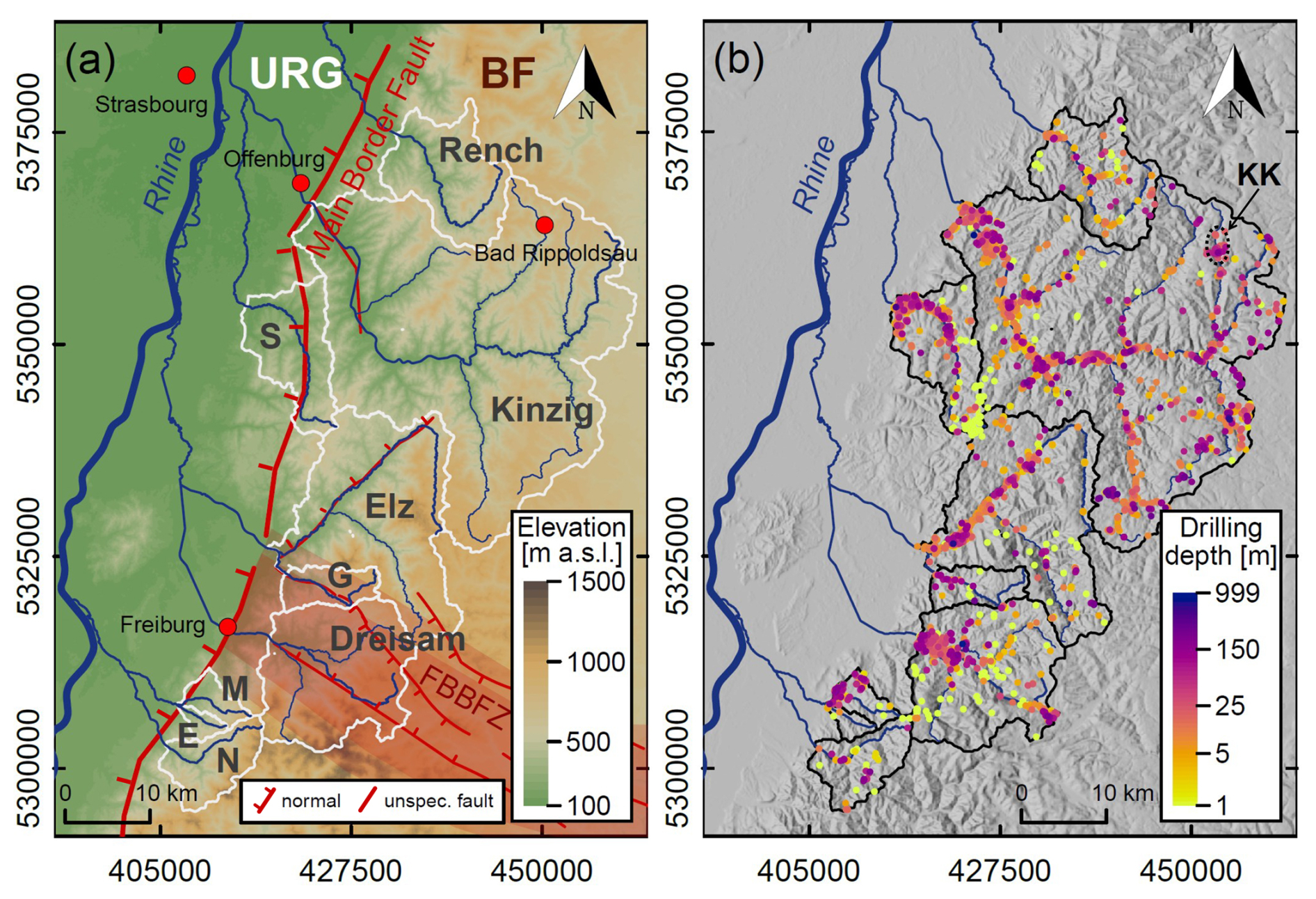
Figure 1 (a) Study area overview including the catchment outlines, main rivers, and selected towns and cities, as well as the main border fault (simplified), separating the Upper Rhine Graben (URG) from the Black Forest (BF), the Freiburg–Bonndorf–Bodensee fault zone (FBBFZ), and some associated normal faults after Grimmer et al. (2017) and unspecific fault traces (LGRB, 2021). Catchments and river network: LUBW (2022); main border fault: from Michel et al. (2024) after Behrmann et al. (2003); FBBFZ: after Egli et al. (2017); elevation data: SRTM (Jarvis et al., 2008). Catchment abbreviations: S: Schutter, G: Glotter, M: Möhlin, E: Ehrenstetter Ahbach, N: Neumagen. (b) Locations and drilling depths of all boreholes, with the location of the reservoir “Kleine Kinzig” (KK) indicated. Note that the data points partly overlap, with larger values on top.

Catchment shapes and the present-day river network are influenced by tectonic structures and complex small- to large-scale fault patterns. The Vosges and Black Forest mountains have been uplifted since the early Miocene as eastern and western rift shoulders of the subsiding URG, which forms the central part of the European Cenozoic rift system (Laubscher, 1992; Schumacher, 2002). Thus, the terrain of the greater area (Fig. 1a) is subdivided into the Black Forest, the foothills, and the 30–45 km wide Upper Rhine Plain. The main structure on the eastern margin of the graben is the roughly NNE–SSW trending main border fault which separates the Black Forest crystalline basement from the foothill zone, also termed Vorbergzone, created by a series of interlinked west-dipping faults (Behrmann et al., 2003). Moreover, many valleys and side valleys of Upper Rhine tributaries, for instance the main Elz valley, follow NE- to NNE-oriented crossing faults or subordinate NW-to-NNW striking shears that often can be traced back to the Variscan orogeny (Grimmer et al., 2017; Schumacher, 2002). The NE-to-SW trending Freiburg–Bonndorf–Bodensee fault zone (FBBFZ) is a further important structural feature, which goes back to late Paleozoic time and represents a large crustal-scale deformation zone including a series of faults (Egli et al., 2017). While a tectonic imprint on the study area thus is clear, this study mainly focuses on the upper and middle courses of the Upper Rhine tributaries on the east side of the major eastern border fault, i.e., within the uplifted tectonic block of the Black Forest.

The landscape of the area is mainly hilly to mountainous with > 1.5 km broad alluvial valleys draining towards the Upper Rhine Plain and base levels of about 300 m a.s.l. (Neumagen, south) and about 190 m a.s.l. (Rench, north). The catchments of the southern Black Forest (Dreisam, Neumagen) include the highest elevations (Feldberg 1493 m, Belchen 1414 m) and are generally characterized by steep slopes and deeply incised valleys in predominantly gneiss, porphyr, or granite rocks (Röhrig, 1997). Glacial landforms such as glacial cirques and moraines are restricted to the headwater areas (Hofmann et al., 2022). The middle part of the Black Forest has lower elevations with peaks below 1100 m a.s.l. Particularly at its eastern rim, Triassic sediments, mainly Buntsandstein and Muschelkalk, are still preserved on top of the crystalline basement of gneiss, anatexites, and some granite, while in the western parts, overlying sediments largely have been eroded (Mäckel, 1997).

The valleys of the study area are filled with fluvial deposits of variable thickness and structure, in many parts of the valley sides intermingled with colluvium and periglacial debris and, particularly at the margins towards the Upper Rhine Plain, locally overlaid by loess (Mäckel, 2000). Pleistocene gravels often show an upper layer of younger, barely weathered material and a lower layer of coarser and heavier weathered sediments (Mäckel and Uhlendahl, 2009). In general, these coarse gravels and sands of Pleistocene age are covered by Holocene overbank fines of a few decimeters to a few meters thickness. Depending on the (sub-)catchment, the average thickness of Holocene alluvial floodplain sediments was estimated to be between 0.9 and 2 m (Seidel and Mäckel, 2007). Moreover, Mäckel (1997) and Mäckel and Uhlendahl (2009) observed distinct, mainly climatically induced Holocene erosion and sedimentation phases and an anthropogenic influence on fluvial dynamics and sediment accumulation by intensified land use.

The study area is characterized by a mid-latitude temperate climate superimposed by orographic effects due to its position on the western windward side of the Black Forest. Thus, long-term mean annual precipitation distinctly increases between the lowlands and the mountainous region, as demonstrated for instance by station data (DWD, 2021) of the Kinzig catchment, ranging between about 890 mm (Offenburg) and about 1890 mm (Bad Rippoldsau). A winter precipitation maximum for the mountainous region and the additional influence of snowmelt or rain on snow create a pluvio-nival discharge regime with most high flood discharges between November and March (Bösmeier et al., 2022).

3 Dataset

The LGRB (State Office for Geology, Resources and Mining) Baden-Württemberg compiled an extensive data basis consisting of 7070 data points within the catchments (Fig. 1b), which include different types of boreholes (90.4 %), as well as prospecting pits (Schürfgruben, 5.5 %) and diverse sampling locations (4.1 %) such as surface mining, excavation pits, landfill monitoring sites, and natural outcrops. The dataset is composed of geological information gathered in the course of many decades, with the oldest documents dating back to the 1930s. The surveys were undertaken for various reasons such as ground investigations, e.g., for road construction, individual construction activities, or flood retention measures, the monitoring of contaminated sites, well drilling, or wind park site investigation. In this context, the data points are rather heterogeneously distributed with a particular concentration in the main valleys, where urban centers and the majority of settlement structures and traffic routes are located. Basic information on these data includes location, name, origin, (usually) the date of recording, a quality rating, and the final depth. In the following, we refer to these points as “borehole data” for the sake of simplicity.

The LGL (State Office for Geoinformation and Land Development) Baden-Württemberg made available a digital elevation model (DEM) in 1 m resolution (LGL, http://www.lgl-bw.de, last access: 12 April 2022; data license dl-by-de/2.0). Based on the provided tiles, catchment DEMs were compiled and resampled to 8 m grid resolution for faster processing, and sinks were filled following Wang and Liu (2006). Moreover, a geological overview map of the area at a scale of 1 : 50 000 and information on tectonic structures were provided by the LGRB (LGRB, 2021). The utilized basic hydrological data include basic and aggregated catchment shapefiles and information on the river network (LUBW, 2022). Data processing and analysis procedures were carried out using R, version 4.4.0 (R Core Team, 2022; http://r-project.org, last access: 25 June 2025), QGIS, version 3.28.11 (http://qgis.org, last access: 24 April 2025), and SAGA GIS, version 8.1.3 (http://saga-gis.org, last access: 25 June 2025; Conrad et al., 2015; Schillaci et al., 2015).

4 Methods

Our aim is to estimate the overall storage volume and spatial distribution of fluvial sediments per catchment based on the available information on sediment cover above bedrock and catchment characteristics, following the preparation and analysis of borehole data and definition of valley floor extents (Sect. 4.1.1 and 4.1.2). As a first benchmark, we approximated expectable ranges of sediment cover by using several suitable valley cross sections throughout the study area (Fig. 2, method A; Sect. 4.2). Taking into account metrics such as the borehole positions within the valley floor, we moreover estimated sediment depths spatially resolved by catchment-specific linear and random forest regression modeling (method B; Sect. 4.3).

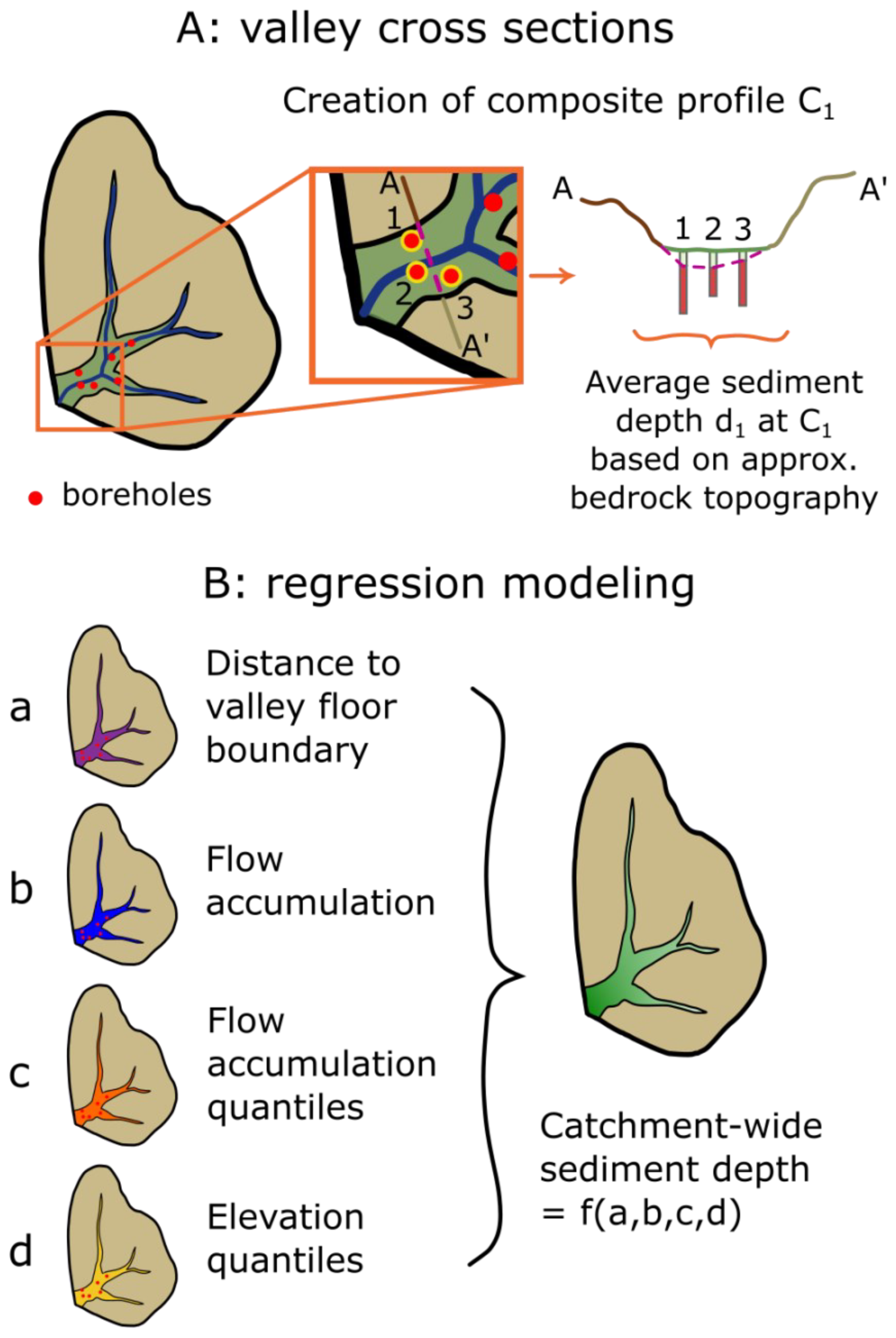
Figure 2 Fluvial sediment volumes were estimated based on a two-dimensional approximation of subsurface bedrock topography at composite profiles and also by using regression modeling of sediment depths by catchment characteristics with models trained on information at borehole locations.

4.1 Preprocessing

4.1.1 Borehole data processing

For most borehole points, more or less detailed information on stratigraphy and/or petrology was provided either as digitized documents in PDF format (roughly 80 %) or as digital spreadsheet (roughly 20 %). The digitized documents often include a combination of different data types such as borehole profiles or graphs with symbols (Signatur), color, descriptions, or abbreviations (Kürzel) indicating the petrography or lists of more or less detailed descriptions of the single layers. The digital, spreadsheet-formatted data contain, inter alia, lists of all layers of the drillings with depth indication and specification of stratigraphy, often petrology, and occasionally provenance or color. Hence, information was gathered either by visual inspection of borehole graphs/profiles or, where documented, utilizing the available stratigraphic or petrologic details.

To obtain information on fluvial sediment depth, we extracted the upper limit of (weathered) bedrock from the borehole profiles or – if the drillings did not reach the bedrock – at least noted the minimum sediment depth. The reliability and level of detail appeared to be very heterogeneous within the dataset, apparently mainly depending on the respective project or the creators of the geological assessment. Considering this broad range of data quality, we focused on differentiating between sediments in general and underlying bedrock.

Moreover, we rated the quality of the borehole data. The available information generally allowed categorization into “precise” data, “imprecise” or “uncertain” data, unusable “bad quality” data, or missing information. To be more specific, in the case an imprecise data range instead of precise information on the sediment–bedrock transition could be extracted, upper and lower ranges were noted. Furthermore, information on (minimum) sediment depth was marked uncertain if the information in digitized documents was unclear, if it showed distinct inconsistencies, or if digital information indicated data uncertainty. Borehole points classified by the LGRB with the poorest data quality were marked as unreliable bad quality data.

Finally, the provided data on borehole top ground surfaces occasionally appeared flawed. Thus, elevation data at the borehole locations were extracted from the high-resolution DEMs and borehole depth information was adjusted accordingly. Besides that, all borehole points along the embankment or within the reservoir “Kleine Kinzig” in the upper part of the Kinzig valley (Fig. 1b) were excluded from the analysis assuming a significant effect of the dam on sediment accumulation.

4.1.2 Valley floor definition

In our evaluation of the spatial distribution of fluvial sediment deposits, the mapping of valley bottoms represented a necessary step. Valley floor areas were defined for the study area catchments utilizing the multi-resolution valley bottom flatness (MRVBF) algorithm (Gallant and Dowling, 2003). The algorithm determines valley bottoms as low and flat areas within their vicinity at multiple scales and produces a continuous index with larger values corresponding to flatter and larger valley floors.

MRVBF computation was carried out per catchment as implemented in SAGA, with default options and an adjusted initial slope threshold of 64 % to comply with the higher DEM resolution of 8 m as compared to Gallant and Dowling (2003), who utilized a resolution of 25 m. A morphological filter with a kernel radius of three cells was applied to close small gaps. For the whole process of valley floor definition, a range of parameter values, such as the initial slope threshold or the relevant MRVBF index values, had to be determined. We chose the best parameter set per catchment – with a special focus on the trunk valleys as major accumulation spaces – by visually comparing the resulting valley floor area and the extent of Quaternary valley fill in the geological overview map by the LGRB.

Valley bottoms were defined as areas with a MRVBF index above the 0.9 quantile, and relatively low vertical distance to the channel network, namely below the 0.4 quantile for the Dreisam catchment and the 0.1 quantile for all other catchments. Therefore, the channel network was computed with a top-down flow accumulation utilizing the Deterministic 8 approach after O'Callaghan and Mark (1984) for flow routing, using 0.3 km² for channel initiation (0.15 km² for the Dreisam catchment).

When choosing the best parameter sets, it turned out to be crucial to find a balance between the best possible representation of valley bottoms in the lowlands and good enough results for the highlands. In some regions with rather flat high plateaus, however, a limitation based on the vertical distance to the channel network was not sufficient as a corrective measure. There, high MRVBF values were assigned to flat ridges or plateaus in headwater areas, such as upland bogs, indicating extensive valley bottoms. To prevent an overestimation of fluvial sediments, it finally appeared necessary to replace MRVBF-defined valley floor areas of the Dreisam catchment with information from the geological maps for areas above the 0.4 quantile of elevation. Besides that correction, across the entire study area, isolated gaps in the mapped valley bottom originating from local small-scale roughness within the valley, such as elevated railway tracks, traffic routes or single buildings, were closed, i.e., deleted, automatically.

4.2 Valley fill estimation based on valley cross sections

Benchmarks of approximate valley fill volumes were computed based on a series of composite valley cross sections spread across the study area and different scales, depending on available borehole locations. Composed of a single drilling up to several adjacent boreholes reaching the bedrock, the cross profiles allow for approximating local bedrock topography and hence the sediment infill. On this basis, a first rough estimation of the valley fill volume of every catchment was derived from the total size of the catchment valley bottom areas and the average sediment covers as observed in all gathered valley cross sections (compare Fig. 2).

As a preparatory work, for every borehole point within the valley floor, an elevation profile across the floor normal to the local valley direction was determined based on code. Here, utilizing the DEM and grids of mapped valley floor, the best transect direction was defined as both crossing the valley floor as directly as possible and traversing the borehole point and the valley centerline at a preferably direct way. Visual inspection of catchment maps and profile positions, first, and the valley transects showing surface topography and the data of the associated boreholes, second, followed. The directions of single profiles across the valley were adjusted manually where considered necessary.

In a next step, locations were selected at favorable valley sections where (1) several adjacent boreholes reaching the bedrock are available and (2) the data points ideally are spread across the valley to provide insight into cross-valley subsurface morphology. In headwater areas, where borehole data are generally scarce, single data points located close to the valley centerline were selected to improve the prospects of approaching the maximum sediment depth and thus a realistic cross section despite only one borehole per profile.

In order to derive a valley cross section C_a from one to several related data points in close proximity, an approach inspired by the construction of curvilinear swath profiles (e.g., Telbisz et al., 2013) was used. With the valley centerline as swath midline and sampling points along individual transects through neighboring boreholes – which may cross the valley at slightly different angles – a composite valley cross profile showing the approximated valley floor subsurface morphology was constructed (Fig. A1). Therefore, instead of computing summary statistics from the transects, the surface elevation and sediment depth data from the borehole points were simply put together, as described in the following and in detail in Appendix A. The borehole positions within the composite profile were determined by the points' relative positions along the respective transects valley floors. The valley floor width W_a of a composite profile is the median of the individual transect valley floor widths. Its direction across the valley is the direction of the central individual transect so that the resulting cross section lies approximately normal to the valley direction. Finally, its position on the map was determined from the mean of x and y coordinates of middle points of the most distant individual transects.

For estimating the cross-sectional area $A_{C_{\mathrm{a}}}$ of the sediment infill of a valley cross profile C_a composed of n boreholes, the profile was split into n+1 sections. In the case of a profile from a single data point, two triangular areas between the borehole sediment depth above bedrock and the distances to the edges on both sides of the valley bottom were computed. For n>1 boreholes, two triangular areas on both valley floor sides and n−1 trapezoids between the borehole sediment depths were added up. Here, the horizontal distances between the borehole points were extracted from the relative positions of the boreholes (i.e., on their respective transects within the valley floor) and projected on the hypothetical valley cross profile with median valley floor width W_a and median direction across the valley. For each valley cross profile C_a, the average sediment depth d_a is defined by

$$\begin{array}{}\text{(1)}& d_{\mathrm{a}}=A_{C_{\mathrm{a}}}/W_{\mathrm{a}}.\end{array}$$

Finally, the valley fill volume V of a specific catchment was approximated by the product of the catchment valley floor area A and all average cross-section sediment depths:

$$\begin{array}{}\text{(2)}& V_{\mathrm{1},\mathrm{\dots },m}=\left\{A\cdot d|d\in D\right\},\end{array}$$

where D is the set of average cross-section sediment depths of all m cross profiles (Eq. 1) defined as

$$\begin{array}{}\text{(3)}& D=\left\{d_{\mathrm{1}},\mathrm{\dots },d_m\right\}.\end{array}$$

4.3 Valley fill estimation based on morphometric modeling

To approximate sediment depths in the valleys, we modeled them as a function of morphometric and hydrologic variables. Therefore, selected metrics were computed, and linear and random forest regression models were fit utilizing the borehole dataset. Finally, catchment-wide valley fill sediment volumes were estimated by applying the most adequate models to the catchment valley bottom areas.

4.3.1 Predictor variables

Catchment morphology, drainage network, and hydrology – along with relevant independent variables, such as initial relief and geological and climatic characteristics – significantly influence channel morphology and deposited fluvial sediments (e.g., Schumm, 1977). A meaningful model to spatially estimate valley fill sediment depth should consider factors that are known to play a major role in shaping present valley subsurface geometries. In this respect, and on the basis of key data utilized in previous studies on valley infills (Sect. 1), we selected a manageable set of predictor variables that mainly reflect some aspects of channel morphology, drainage pattern, and relief. In order to visualize catchment-specific characteristics and assess the representativeness of the available data within each catchment, we used empirical cumulative distribution functions (ECDFs; see Supplement, Fig. S3).

(a) Distance to the valley floor boundary

For every catchment, a grid indicating the distance to the valley floor boundary for all cells within the valley bottom (compare Sect. 4.1.2) was prepared. Therefore, at first, a grid (8 m resolution) indicating the border of the valley floor was created. This “border mask”, displaying cells inside, yet at the margin of the valleys, was computed on the basis of a grid where a cell value of 1 indicates areas within the valley floor, a value of 0 the catchment area surrounding the valleys, and NA values the area outside of the catchment. Note that at the catchment outlet, where the catchment boundary truncates the valley floor, the border mask grid has a gap; otherwise, the artificially defined catchment boundary would lead to artificially decreasing values of the predictor variable at the outlet.

For every cell inside the area defined as valley floor, the distance to the valley boundary was then determined by the minimum of the Euclidean distances between the cell and all cells at the valley margins (i.e., border mask values of 1).

(b) Flow accumulation

To be able to relate deposited fluvial sediments with the upstream contributing area, the flow accumulation values had to be “spread” across the valley floors. This is because the maximum flow accumulation values, which represent the relevant contributing area for sediment generation, accumulate in single channels, whereas fluvial sediments cover the entire valley floor, which is therefore of relevance.

At first, catchment flow accumulation was computed utilizing a top-down approach and the D8 algorithm after O'Callaghan and Mark (1984) as implemented in SAGA. Then, flow accumulation values across the valley floor were computed using an algorithm (see Appendix B).

(c) Flow accumulation quantiles

Moreover, grids of quantiles of flow accumulation across the valley bottom (8 m resolution) were prepared on the basis of predictor variable b. Therefore, based on a random sample of 10 % of the data excluding NAs – to keep computing time at a low level – a lookup table was created showing flow accumulation values across the valley floor and their respective quantiles by steps of 0.001 for every catchment. For the quantile grid, the respective quantiles were extracted from this table for all grid cells within the valley floor.

(d) Elevation quantiles

Grids of elevation quantile values for the valley bottom area were prepared on basis of the catchment DEM at 8 m resolution. Therefore, 10 % of all elevation values of a specific catchment were sampled, a lookup table of elevation associated with the quantiles of these values by steps of 0.001 was created, and for all grid cells within the valley floor, the respective elevation quantiles were extracted.

4.3.2 Valley fill sediment depth estimation by regression modeling

Data processing prior to modeling consisted of repeated stratified sampling and a random split of the database in 80 % training and 20 % validation data for the respective areas. Due to a clustering of boreholes, e.g., in cities or along roads (Fig. 3), and subsequent overrepresentation, spatial autocorrelation sampling bias has to be taken into account (e.g., Reddy and Dávalos, 2003). In order to reduce this bias, a stratified sampling approach, in this case filtering by a distance-based spatial thinning, was used before splitting the data into training and validation sets: here, data points were repeatedly (n = 250) randomly selected from the dataset, and subsequent to every selection, boreholes in close (< 10 m) proximity to the selected borehole were removed from the remaining dataset. To examine the effect of uncertain and imprecise information, not only precise borehole data were utilized for modeling but also datasets including the data points marked as “uncertain” and “imprecise” (Sect. 4.1.1). For the latter, only a possible range of sediment depth above bedrock was given; thus values within the respective ranges were randomly selected during each data sampling repetition.

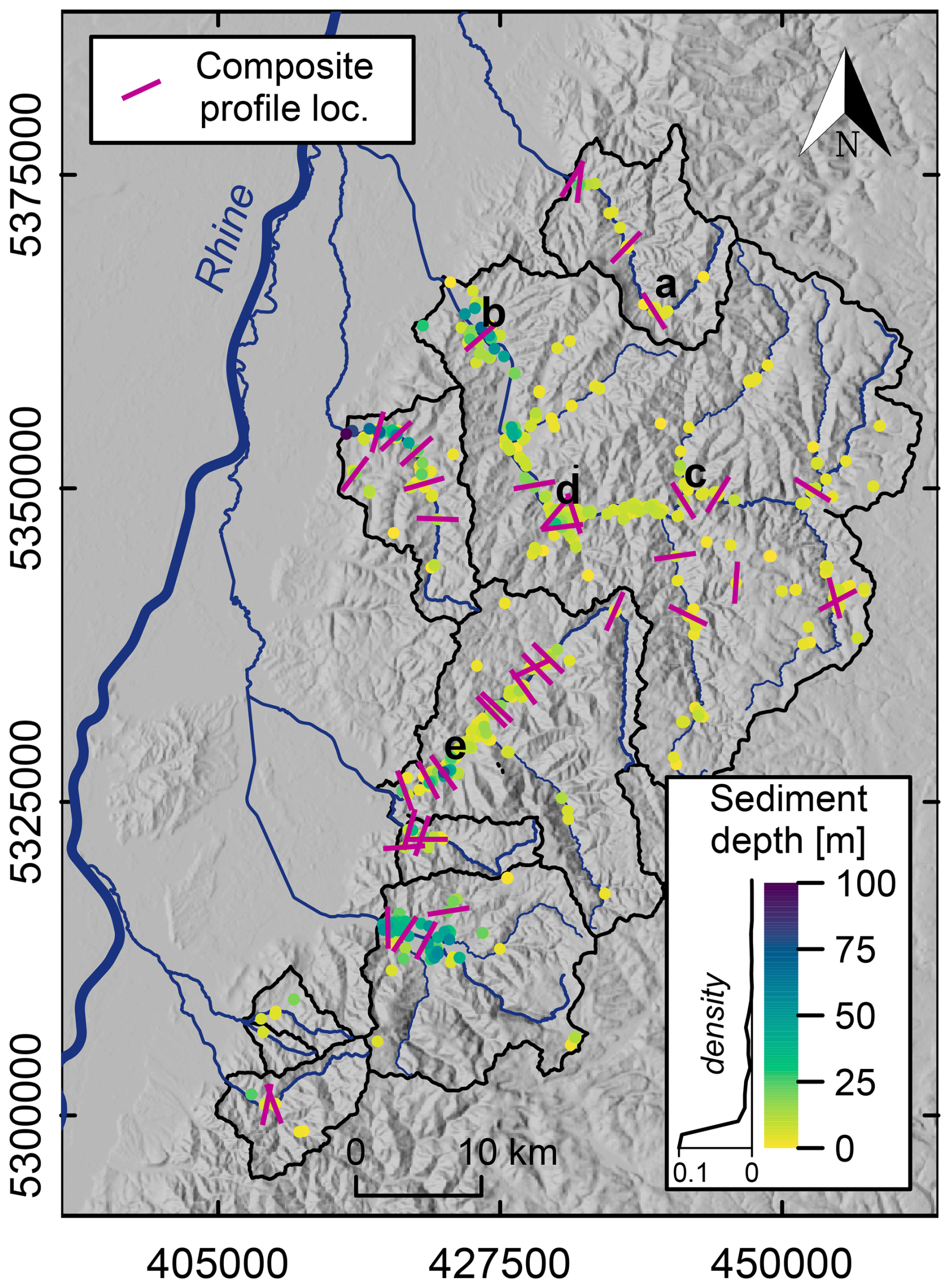
Figure 3 Sediment depth above bedrock of all 978 borehole points within the valley floor areas – including uncertain and imprecise (minimum depth) information – with catchment borders, main rivers (compare Fig. 1a), and data density distribution indicated. Note that the data points partly overlap, with larger values on top. Locations and positions of composite profiles are marked as well, and refer to Fig. 4a to e. Catchments and river network: LUBW (2022); elevation data: SRTM (Jarvis et al., 2008).

Simple and multiple linear regression models with sediment depth as response (output variable) and the metrics a to d (Sect. 4.3.1) as predictors (input variables) were then fit to the data catchment-wise and for the entire study area. For model selection, Akaike's Information Criterion (AIC; Akaike, 1973), variable significance, and the model fit measured by the adjusted R² were consulted. Moreover, model performance was assessed by applying the models to validation datasets and calculating the root mean square error (RMSE) as well as by visual inspection of diagnostic plots showing observed values plotted against fitted values and residuals (the difference between observations and predictions) plotted against fitted values.

Additionally, random forest regression modeling, which is a machine learning technique that combines a number of models and can thereby achieve a higher predictive precision, was explored. Here, we used the R package “randomForest” (Liaw and Wiener, 2002) which implements the algorithm by Breiman (2001). A random forest regression model is constructed by an ensemble of regression trees using bootstrap aggregation, where each tree is trained on a random sample of the training data with replacement. Thereby, the package “randomForest” allows a post hoc evaluation of variable importance by randomly permuting each predictor's values in the out-of-bag data and measuring the resulting increase in mean square error of the prediction.

Random forest regression is commonly utilized in studies with high-dimensional datasets that might include irrelevant or interacting variables. Nevertheless, its value has also been shown in cases of a low feature number (Luan et al., 2020; Zavareh et al., 2024), particularly as random forests are more effective than linear models in handling complex, potentially nonlinear relationships typical of environmental data.

For our study, we built random forest models with a tree number of n = 500 with sediment depth as response and up to four predictor variables in possible combinations, as presented in Sect. 4.3.1. Models were repeatedly (n = 250) fitted to the training datasets and applied to the validation sets, using the stratified random sampling approach as described above. Utilizing these resampling results, the models were assessed and selected: for diagnostics, an analysis of explained variance and the RMSE as goodness-of-fit measures, a visual inspection of residuals plotted against predicted values of training and validation datasets, and an inspection of observations versus model predictions were combined. The explained variance was computed as follows:

$$\begin{array}{}\text{(4)}& \mathrm{expl}.\mathrm{var}.\left[\mathit{\%}\right]=\mathrm{100}\cdot \left(\mathrm{1}-{\displaystyle \frac{\mathrm{var}\left(y-\widehat{y}\right)}{\mathrm{var}\left(y\right)}}\right),\end{array}$$

where $\mathrm{var}(y-\widehat{y})$ is the sample variance of the residuals and var(y) is the sample variance of the results in every sampling repetition. The RMSE (0.25 quantile, median, and 0.75 quantile) as well as the diagnostic plots were moreover utilized to compare linear with random forest model performance.

4.4 Sediment volume computation

The selected linear and random forest model structures were applied repeatedly, as described above, to the associated areas in order to estimate sediment volumes for each catchment. Therefore, in every random sampling repetition, sediment depth estimates were computed for every grid cell of a catchment. Catchment sediment volumes are then the result of multiplying the sediment depths with the cell area (8 m × 8 m) and subsequent addition over the catchment valley floor area. Moreover, the ensemble (here: median values of sediment depth per grid cell) of all sampling repetitions was computed per catchment to create result grids and for spatial visualization purposes. Where appropriate, the effect of borehole data imprecision and uncertainty was examined by comparing the results based on precise data with the datasets enriched by imprecise and uncertain data.

5 Results

5.1 Borehole data within the valley floors

Preprocessing of the provided borehole dataset from the LGRB (Fig. 1b) revealed that about a third of the 7070 data points could be used for further processing. The majority of the data were discarded because the drillings did not reach the bedrock (32.2 %), insufficient information on borehole points was given (34.3 %), or the data quality was poor (0.8 %).

Table 1 Catchment specifics, including details on utilizable (precise, imprecise, and uncertain) boreholes reaching bedrock within the valley floor, information on composite valley cross sections, and resulting valley fill volume estimates.

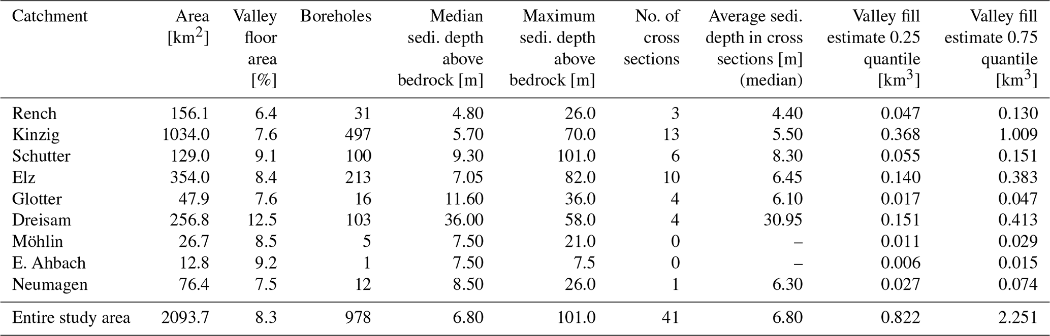
The mapping of valley floors using the MRVBF index resulted in a total valley floor area of 175 km², which is 8.3 % of our study area covering 2094 km² (Table 1). Therein, the large Kinzig catchment comprises most of these areas (45 %), followed by Dreisam (18 %) and Elz catchments (17 %). With regards to the share of valley floor area on catchment area, the Dreisam, with its large tectonically controlled “Zarten basin” structure, contains the highest percentage (12.5 %) and the Rench catchment the lowest (6.4 %). The maximum valley widths of the nine studied catchments extend between about 400 m (Möhlin) and 3 km (Dreisam).

Merging the results from borehole data preprocessing and valley bottom definition, it becomes apparent that only a small proportion of the initial dataset can be used for valley fill sediment estimation. In addition to missing or unreliable data or drillings too shallow to reach underlying bedrock, many drillings have been undertaken beyond the valley floors. Hence, only 13.8 % (978 out of 7070) borehole data points provide information on sediment thickness within the valley bottoms, among them 76 uncertain and 35 imprecise data points, which is about 10 % of the utilizable data. Apart from a preferred concentration of these points in the main valleys and towards the Upper Rhine valley, the proximity to settlement structures plays a role regarding the distribution within the different catchments (Fig. 3). While a large percentage of the data represent rather thin sediment coverage (0.5 quantile of 4.9 m, 0.9 quantile of 22.0 m), the total range extends from 0 to 101 m, and 3 % of the drillings indicate sediments > 45 m thick. These locations of rather thick sediment cover are predominantly situated in the valleys of the lower reaches of Kinzig, Schutter, Elz, or Dreisam. The largest number of data points are located in the Kinzig catchment (51 %), followed by Elz (21 %), Dreisam (11 %), and Schutter (10 %; compare Table 1). The data density of boreholes per catchment km² ranges between 0.08 (Ehrenstetter Ahbach) and 0.78 (Schutter). With regard to the representativeness of the borehole data in relation to key information (elevation, flow accumulation, distance to the valley floor boundary) underlying the selected predictor variables (Sect. 4.3.1), it appears to depend on the catchment and the specific characteristic but also on the sample size (compare Fig. S3, Supplement). For instance, in the Kinzig catchment, the available boreholes cover almost all altitudes where the valley floor is located, while borehole data in the Elz catchment tend to occur more in lower altitudes despite an overall rather high number of data points.

5.2 Valley fill geometry from cross sections

A total number of m = 41 composite valley cross profiles, each containing information from one to 12 (median: four) different borehole points, was compiled to obtain an initial estimation of the valley fill volume in the study area (compare Fig. 6 and Supplement, Table S2). Suitable locations for composite profiles (particularly for those including several boreholes) could be found mainly at places where the borehole density is comparably high, i.e., in the main valleys with a tendency to middle-to-lower catchment parts (Figs. 3 and S1). Likewise, the distribution of the cross sections among the different catchments roughly follows the relative quantity of useful boreholes (Table 1).

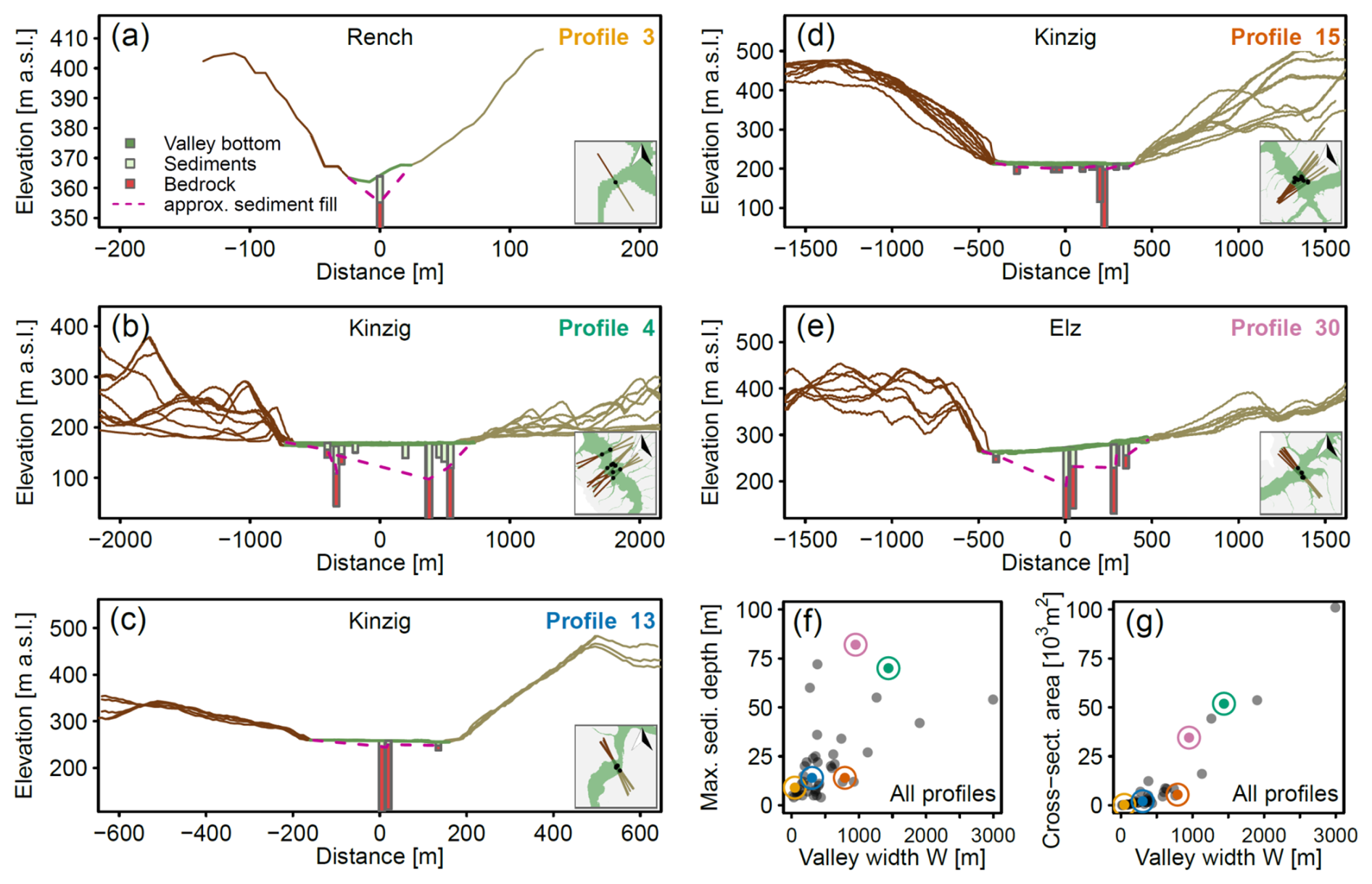
Figure 4 (a–e) Selected valley cross sections (compare Fig. 3), composed of one or more transects through boreholes, showing the approximated bedrock topography in the valleys. The x axis zero positions mark the middle of the valleys; x and y axis scaling is moreover tailored to the respective valley dimensions. (f) Maximum sediment depths and associated valley floor widths (median of included transects) of all composite profiles. (g) Cross-sectional area of approximated fluvial sediment fill per cross section.

While the majority of the cross sections are located within the main valleys with widths between 100 and 1000 m, a few profiles cross rather narrow headwater side valleys, and three profiles (38–40; see Supplement, Fig. S2) stretch across the up to 3 km wide Dreisam basin. Overall, valley floor widths vary between 16 and 3 km, with an interquartile range of about 190–630 m (Fig. 4f).

An overview of the variety of valley shapes, presenting details on selected composite cross sections in the Rench, Kinzig, and Elz catchments, is given in Fig. 4. Profile 3 shows one of three profiles (3, 19, 23; see Fig. S2) in upland areas across rather narrow valleys, with a valley floor width < 50 m (Fig. 4a). Even though this cross section is based on a single borehole only, it appears reasonable to assume a rather V-shaped valley fill geometry, and it thus is related to a comparably deep sediment fill in relation to the narrow valley. However, in headwater areas of the study area, relatively shallow sediment infills can be found as well; e.g., see profile 20 in the Kinzig catchment (see Fig. S2).

Profiles with shallow sediment bodies lacking clear depth variations are representative of nearly half of the compiled cross sections that contain enough information, i.e., drilling points across the valley floor, to allow a reasonable statement about the approximate shape of the bedrock topography (Fig. 4c and d).

In contrast, the other half of the cross profiles rather demonstrate deepening towards the middle of the valley. The cross sections in Fig. 4b and e, for instance, suggest a deeply incised, box- or V-shaped valley, partly with asymmetric bedrock topography and presumably substantial (tens of meters) jumps. Larger variations in sediment depth, which might indicate vertical displacements of the bedrock, can also be observed in a couple of other cross sections in Fig. S2 (Supplement), particularly in the Schutter (profiles 5 and 6), Elz (profile 31), Dreisam (profile 38), and Glotter (profiles 33 and 34) catchments. Examples of a relatively symmetric and – with regard to the large dimensions – smooth bedrock topography are profiles 38–40, across the wide Dreisam basin. Finally, strongly asymmetrically steep valley sides may be but are not necessarily associated with asymmetry of the approximated valley fill geometry and/or an inclined valley bottom (e.g., Fig. 4e and profiles 16, 20, 21, 27, Fig. S2).

A comparison between the maximum sediment depths observed in the cross sections and the associated valley widths demonstrates a wide spread but also suggests that (> 1000 m) wide valleys tend to contain at least 15 to 25 m of maximum sediment depth (Fig. 4f). The average sediment depths $d_{\mathrm{1},\mathrm{\dots },m}$ of the composite valley cross profiles comprise a range from 2 to 36.3 m. When comparing the median values of d per catchment, it is moreover striking that the Dreisam clearly stands out with about 30 m, which is a result of the comparably wide and deep sediment cover of the main basin (see Table 1 and Fig. 3).

5.3 Model selection

Both linear and random forest regression models show good model fits for Rench, Kinzig, and Schutter with adjusted R² values between 0.52 and 0.74 and about 60 %–80 % of the variability in sediment depth explained, respectively (Tables 2 and 3; Fig. 5). However, for all catchments except for Glotter and Möhlin, model performance measured by the RMSE (0.25 quantile, median, and 0.75 quantile) is slightly to considerably better in random forest than in linear regression models. This is particularly true for the Dreisam (median RMSE of 15.05 vs. 9.40) and can also be seen in the diagnostic plots (Fig. 5).

Table 2 Metrics (selection) on the performance of the selected linear models, here based on 250 sampling repetitions. Note that the adjusted R² of marked (^∗) catchments is based on the entire dataset, while the RMSE was computed based on the validation sets within the specific catchments only.

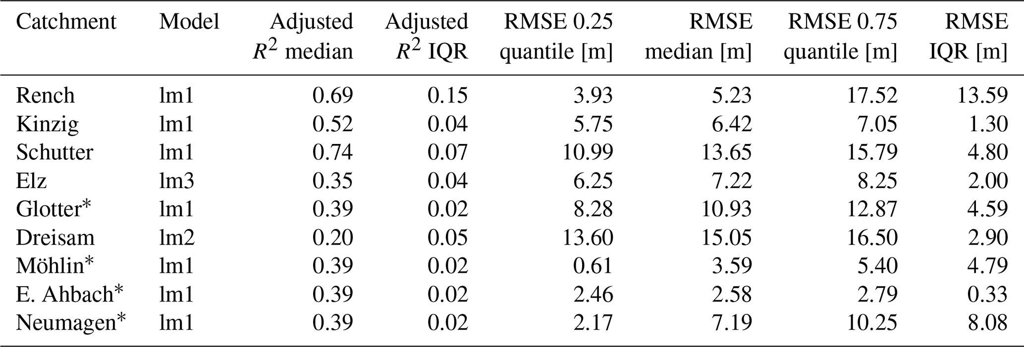
Table 3 Metrics (selection) on the performance of the selected random forest models, here based on 250 sampling repetitions. The explained variance of marked (^∗) catchments is based on the entire dataset, while the RMSE was computed based on the validation sets within the specific catchments only.

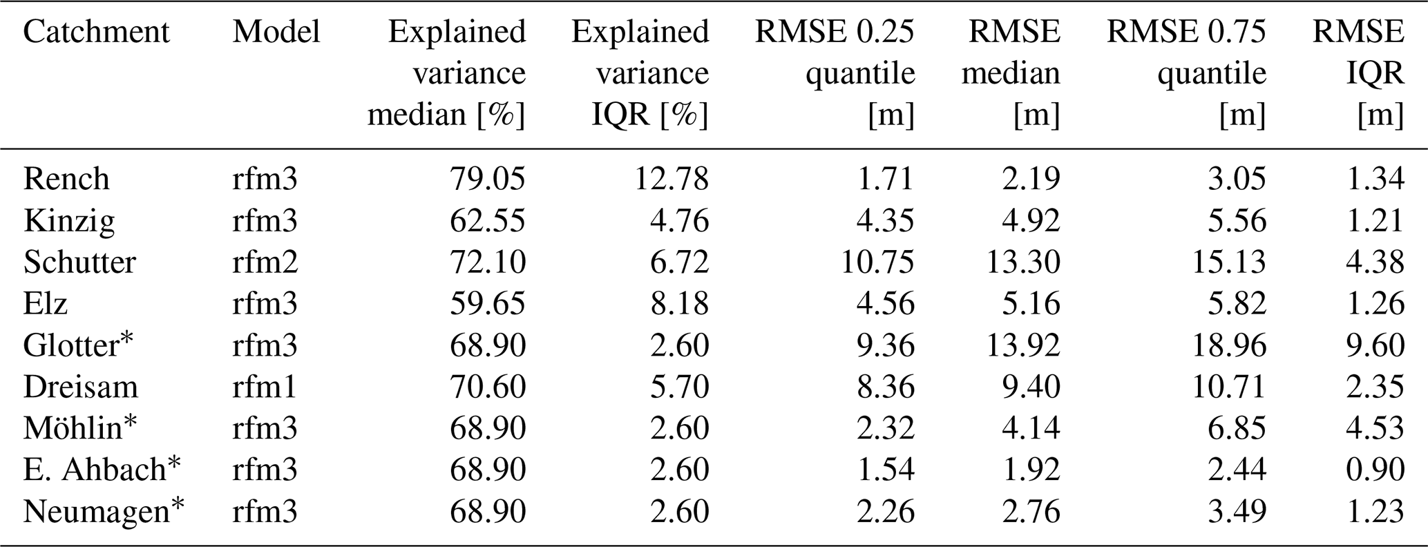
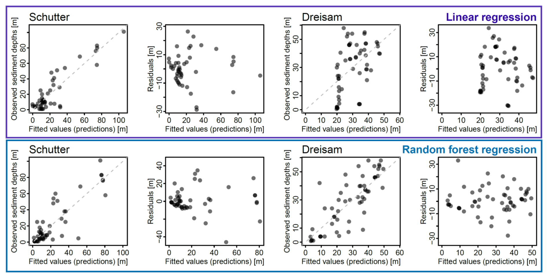
Figure 5 Selected diagnostic plots by the example of Schutter and Dreisam for random validation datasets, showing predicted in comparison to observed values and the 1 : 1 line (left) and associated residuals (right) for both catchments for the selected models, on the top for linear regression and on the bottom for random forest regression modeling.

To be more specific regarding the results of the model selection progress: for the exploratory analysis of linear regression models per catchment, precise borehole data points with information on sediment cover above bedrock within the valley bottoms were utilized and repeatedly sampled (replication size = 10) to exclude drillings within less than 10 m proximity (see Sect. 4.3.2). The best model structures were selected via forward model selection so that the predictor variables a to d as defined in Sect. 4.3.1 as well as variable combinations and interactions were included step by step to form more complex models. By visually checking for obvious patterns in the diagnostic plots, tagging model parameters with a p value > 0.1, and comparing the relative changes in explained variance and AIC of different models, variables were excluded again, so that a set of three models remained, including the best model for every catchment, evaluated using the “precise data” sets. Variable transformation, here utilizing the square root or square of input variables, did not result in significant improvements. The final model structures were defined as follows:

• lm1: sediment depth $\sim a\times c\times d$, or in statistical notation $y_i=\mathit{\alpha }+{\mathit{\beta }}_{\mathrm{1}}\cdot a_i+{\mathit{\beta }}_{\mathrm{2}}\cdot c_i+{\mathit{\beta }}_{\mathrm{3}}\cdot d_i+{\mathit{\beta }}_{\mathrm{4}}\cdot a_i\cdot c_i+{\mathit{\beta }}_{\mathrm{5}}\cdot c_i\cdot d_i+{\mathit{\beta }}_{\mathrm{6}}\cdot a_i\cdot d_i+{\mathit{\epsilon }}_i$,

• lm2: sediment depth $\sim a+a:c$, or in statistical notation $y_i=\mathit{\alpha }+{\mathit{\beta }}_{\mathrm{1}}\cdot a_i+{\mathit{\beta }}_{\mathrm{2}}\cdot a_i\cdot c_i+{\mathit{\epsilon }}_i$,

• lm3: sediment depth $\sim a+a:b$, or in statistical notation $y_i=\mathit{\alpha }+{\mathit{\beta }}_{\mathrm{1}}\cdot a_i+{\mathit{\beta }}_{\mathrm{2}}\cdot a_i\cdot b_i+{\mathit{\epsilon }}_i$,

where α and ${\mathit{\beta }}_{\mathrm{1},\mathrm{\dots },n}$ are model parameters and ε_i the errors represented by each observation y_i of sediment depth. The input variable a represents the distance to the valley floor boundary, b the flow accumulation across the valley floor, c the flow accumulation quantiles, and d the elevation quantiles. The model lm1 was selected best model for all catchments except for the Dreisam and Elz, where lm2 and lm3, respectively, appeared better in diagnostics, particularly with regards to heteroscedasticity (Table 2).

The database of four catchments (Glotter, Möhlin, E. Ahbach, Neumagen) was considered too poor for the validation set sampling approach with a sample size of n < 20 that was further reduced due to drillings in close proximity. Hence, lm1, representing the overall best performing model structure, was fit to the entire dataset and used for sediment depths prediction and volume computation in these four catchments. For Schutter, Rench, and Kinzig, the selected models had the highest adjusted R² values, while for the Dreisam, it was as low as 0.20 for the best model. RMSE values appear to be relatively high for some areas, e.g., with median values up to 15.05 m and 13.65 m, respectively, in the Dreisam and Schutter catchments. These are, however, also areas with comparably thick sediment cover in the valley floors (Table 1).

Similarly, for the random forest model selection, an exploratory data analysis was initially carried out using the “precise data” sets to find the best models of sediment depth as the result variable and the variables a to d, as well as their combinations as input variables. With regards to quantitative selection criteria and visual diagnostics, the best model fits could be achieved by the model structures

• rfm1: sediment depth $\sim a\times c\times d$, i.e., a model with input variables a, c, and d,

• rfm2: sediment depth $\sim a\times b\times d$, i.e., a model with input variables a, b, and d, and

• rfm3: sediment depth $\sim a\times b\times c\times d$, i.e., a model with input variables a, b, c, and d.

In particular, according to the explained variance, rfm3 performed best for all catchments but for Dreisam (rfm1) and Schutter (rfm2). However, all three models performed very similar, with small differences only regarding the examined criteria. Other parameter combinations could explain less variance in the data and/or the residuals showed a more conspicuous pattern. Again, the entire dataset was used to fit the three models (rfm3 selected) to predict sediment depth estimates for Glotter, Möhlin, E. Ahbach, and Neumagen, the catchments with a database too poor for the validation set approach.

5.4 Valley fill volumes

The approximations of valley fill volumes by valley cross sections (method A, Fig. 6) indicate that the three catchments Kinzig, Dreisam, and Elz are largest valley fill storage areas within the study area, with about 45 %, 24 %, and 17 %, respectively, of a (median) study area total of 1.2 km³. Likewise, regression modeling (method B, Fig. 6) points to the Kinzig catchment as the largest storage area. With about 1.1 km³ of valley fill sediments compared to the study area total of 2.8 km³, the Kinzig catchment comprises roughly 42 %, followed by the Dreisam (0.9 km³ or 31 %), and the Elz (0.3 km³ or 13 %), based on the median values of linear regression utilizing precise data only. All estimates can be found in the Supplement (Tables S2–S4).

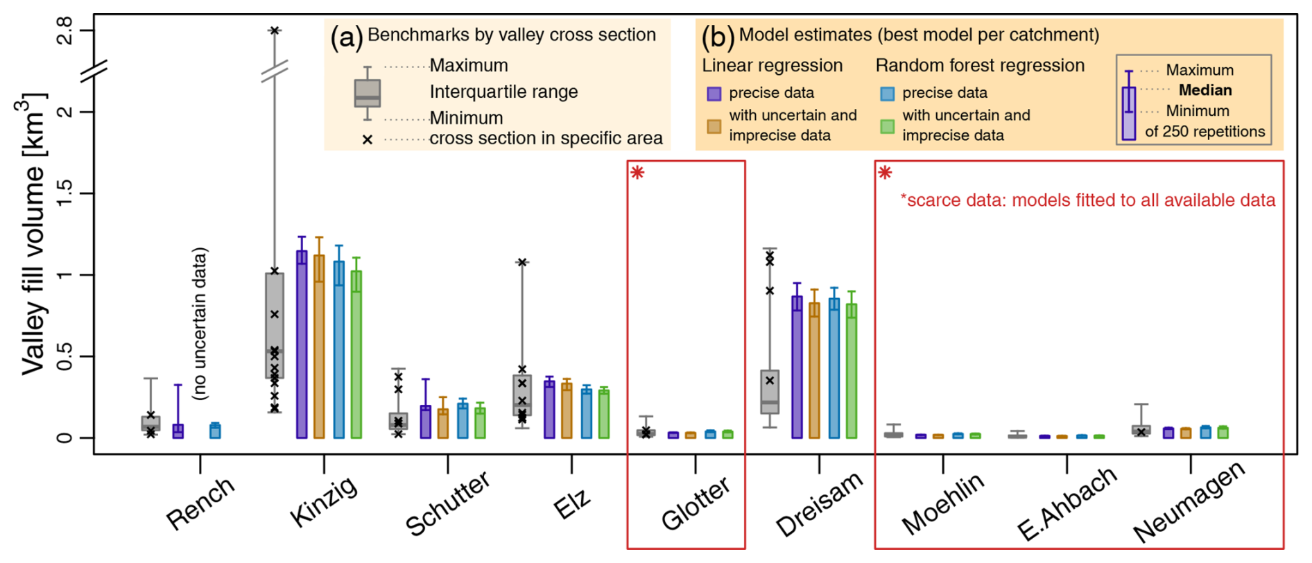
Figure 6 Valley fill volumes computed on the basis of composite cross profiles (method A) and regression modeling (method B). The gray boxplots show $V_{\mathrm{1},\mathrm{\dots },\mathrm{41}}$, which is the whole range of data produced by multiplying the average sediment depths of all 41 approximated cross sections with each catchments valley bottom area. The single data points represent only the data derived from profiles within the specific catchments.

However, the regression model estimates often deviate considerably from the benchmark approximations: for instance, the median values from method B, linear regression (Fig. 7; Supplement, Tables S2–S4), are much higher, particularly for the Dreisam (0.87 vs. 0.22 km³), the Schutter (0.2 vs. 0.08 km³), and the Kinzig (1.15 vs. 0.53 km³). The best agreement is found for the Rench (0.08 vs. 0.07 km³). When comparing the regression model estimates with the approximations by valley cross sections in the particular areas, as marked by “×” in Fig. 6, the compliance between the approaches appears better nevertheless. This may be evidence for the regression models being able to consider the effects of areas-specific valley geometries. As described by Eq. (2), the valley fill estimations utilizing valley cross sections (method A) scale with valley bottom area.

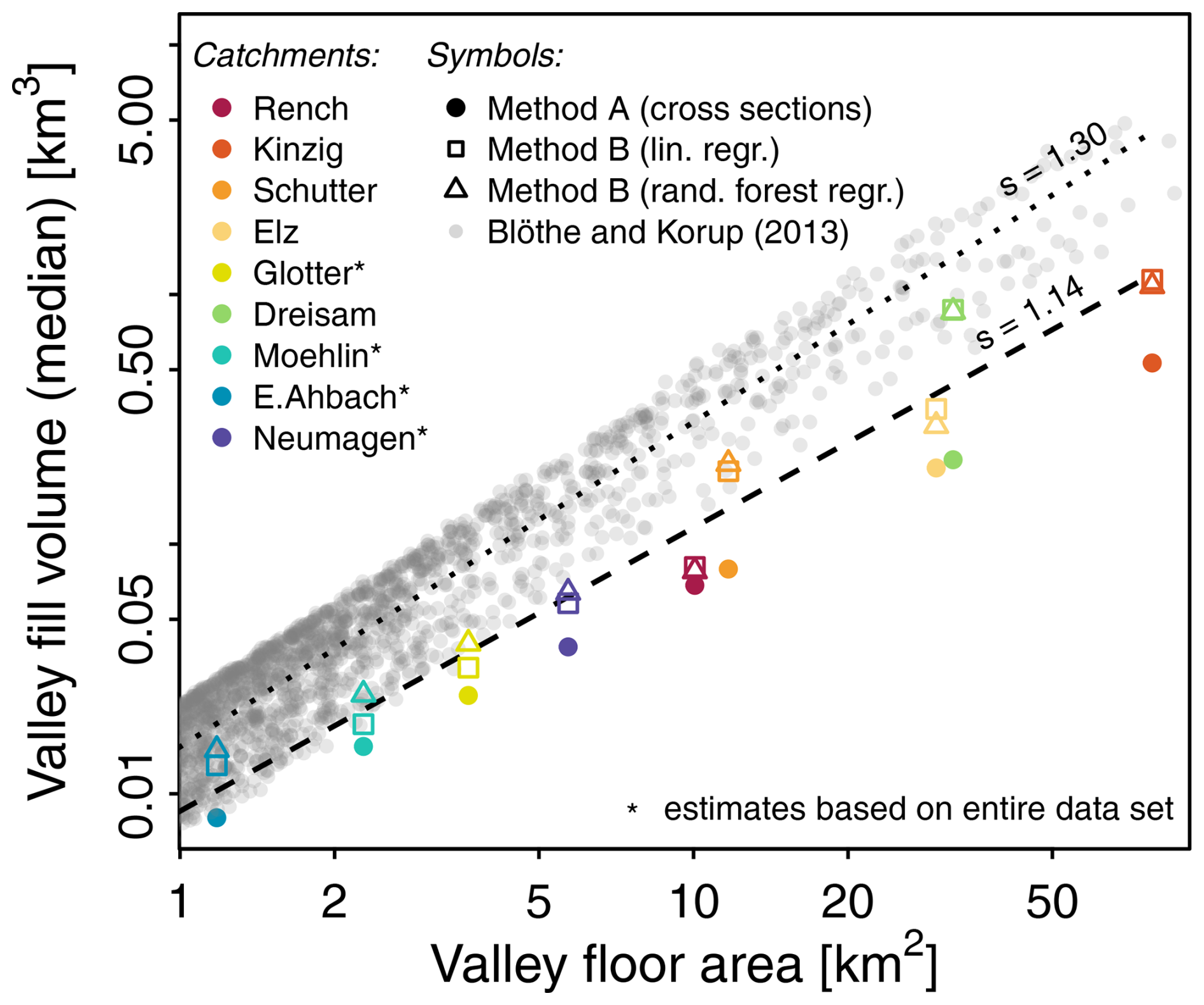
Figure 7 Valley fill volume estimates (median values) computed on the basis of composite cross profiles (method A, compare Fig. 6) and regression modeling (method B, precise datasets) in comparison to published data. Lines with scaling exponents “s” indicated show fitted power-law equations for published data (dotted) and the linear regression estimates (dashed) of this study.

Moreover, for comparative purposes, a power-law equation with the form

$$\begin{array}{}\text{(5)}& V=b\cdot A^s,\end{array}$$

where b is the intercept and s the scaling exponent (e.g., Blöthe and Korup, 2013), was fit (Venables and Ripley, 2002) to the empirical relationship between valley fill volume V and valley floor area A.

While the quantity of valley fill sediments tends to increase with valley floor area, the regression model estimates show a disproportionately high sediment volume for some areas, specifically for the Schutter and the Dreisam. This is well illustrated by their notable positive deviation from the regression line of the associated power law (Fig. 7).

As concerns differences within method B, the linear and random forest models estimates are in good agreement even though random forest model fits are considerably better than those of linear models (see Sect. 5.3). The differences between the results of linear and random forest modeling for the individual catchments are on average around 13 %, whether or not uncertain and imprecise data were included in the analysis. They have a tendency to be larger for small catchments – with the median values of random forest regression being even 32 % (Möhlin) or 25 % (Glotter) higher than the linear regression model results – while they are relatively small for the large catchments of Kinzig (−5.6 %) and Dreisam (−1.6 %). With regards to model results from precise, uncertain, and imprecise data in comparison to using precise data only, the average difference is about 3 times higher in random forest model results than in linear model results (13 % vs. 4 %).

Finally, a spatial visualization of regression model estimates highlights similarities and differences between linear and random forest model results (Fig. 8). In both Fig. 8a and b, rather low sediment depths are apparent in upper and middle catchment parts and thicker sediments in the lower valleys. However, varying patterns of sediment distribution at kilometer to sub-kilometer scales are visible particularly in the lower catchment parts: linear models tend to produce values steadily increasing towards the middle of the valleys while random forest models result in rather continuous areas of similar sediment depth, which are higher downstream and in the valley centers. Hence, random forest regression appears to reproduce the rather shallow to trough-like main valleys more realistically than linear regression, which here has a tendency to form V-shaped valleys.

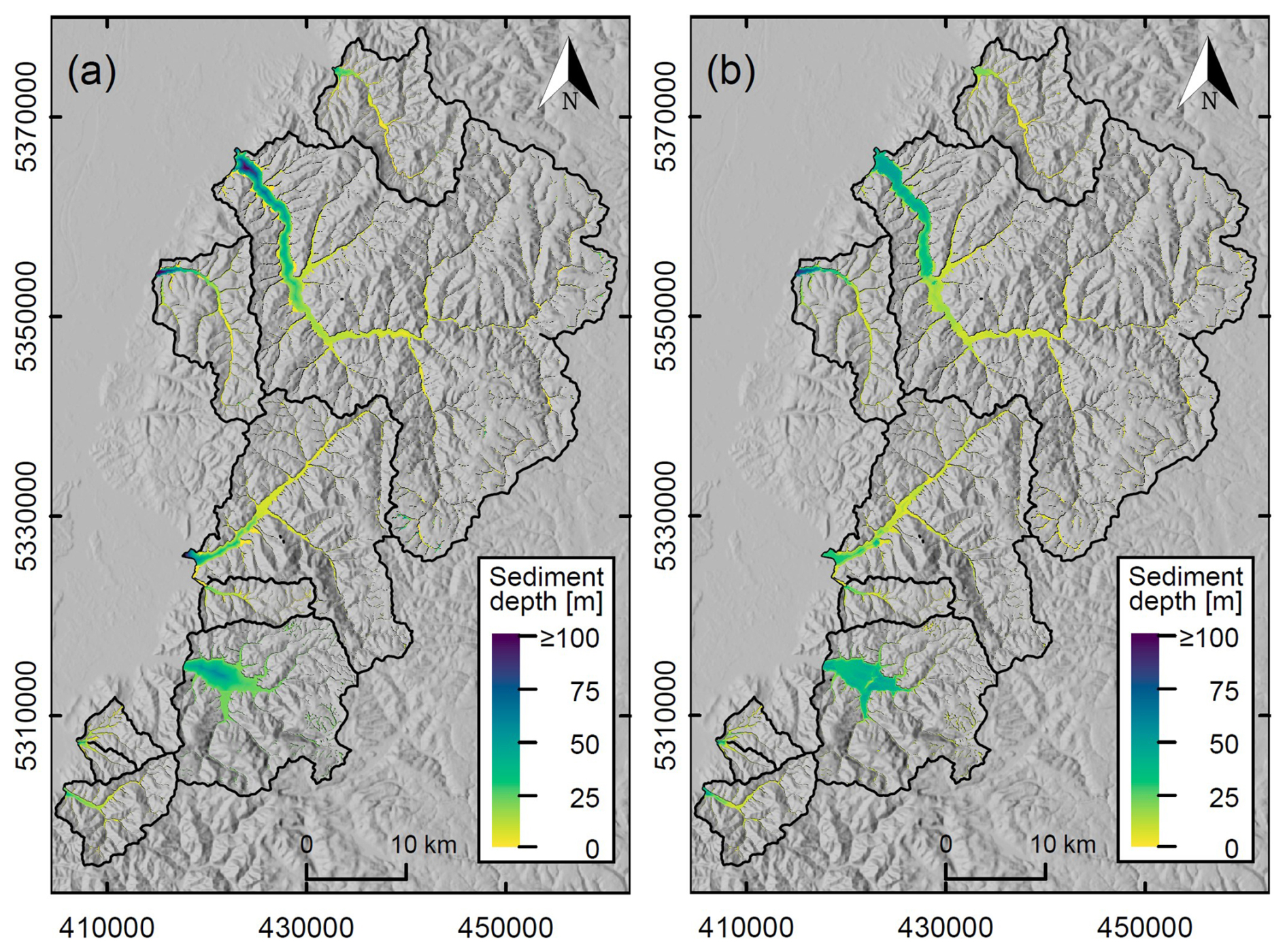
Figure 8 Spatial distribution of linear (a) and random forest (b) regression model estimates. The maps display median values of valley fill sediment depths for each grid cell, based on an ensemble of results from repeated random sampling utilizing precise data and the best model per catchment.

6 Discussion

6.1 Results in contrast to previous literature

We provide the first comprehensive study on sediment storage in alluvial valleys for a large part of the middle and southern Black Forest. Our results can be compared to existing regional studies that focus on geomorphodynamic and (pedo-)stratigraphic analyses, as well as to studies investigating fluvial sediment storage in other regions. In contrast to a comprehensive quantification of sediment volumes stored in Himalayan valley fills (Blöthe and Korup, 2013), the results of our study show smaller volumes per area for most of the catchments and methods, thus a less steep power-law regression line (Fig. 7). Apart from the very different geomorphological and climatic setting of the Himalayas with largely glacigenic valley fills in wide, overdeepened valleys, the volume–area scaling applied by Blöthe and Korup (2013) is based on a similarity between bedrock topography underneath valley fills and the dissected, unburied topography. For most of the trunk valleys in the Black Forest, this assumption would overestimate the sedimentary volume contained in valley fills. Exceptions include the Dreisam, with a wide and deep basin, and the Schutter, with a deeply incised lower main valley (Supplement, Figs. S1 and S2, profiles 39 and 5), which indeed agree well with the values published for Himalayan valley fills. Furthermore, the percentage of the total catchment area covered by valley fills in our study (6.4 %–12.5 %) is considerably smaller than the Himalayan data (11 %–16 %) but better matches estimates of valley fill distribution in the European Alps (Straumann and Korup, 2009), which cover on average 6 % of the basin areas.

Regarding valley cross sections that delineate the subsurface bedrock topography, previous literature is rather scarce and spatially limited, though indicating considerable heterogeneity between and within catchments, which is in agreement with our results. For instance, Mäckel (1997) attests differences in the stratigraphy of fluvial terraces of Black Forest rivers due to varying degrees in erosional and depositional episodes. Connected to more intense fluvial incision towards the border of the Black Forest, in places Pleistocene gravels have been completely or partially removed by the early Holocene. While we did not investigate valley fill stratigraphy, stronger tectonic influence on valley evolution along the main Black Forest border fault (Mäckel, 1997; Mäckel and Röhrig, 1991) may be reflected in the particularly high values of maximum sediment depths in the lower catchment parts of Kinzig, Schutter, and Elz (e.g., Fig. 4b, e, f; Fig. S2, profiles 5 and 6).

Then, Mäckel (2000) examined valleys up until the bedrock within the headwater area of the Schiltach, a Kinzig tributary, and we could compile two cross sections supported by several boreholes for the Schiltach just a few kilometers downstream. Our results (Figs. S1 and S2, profiles 20 and 21) clearly show rather smooth bedrock topography with very shallow sedimentary cover in a gently sloping terrain. This is quite consistent with the trough-shaped valleys originating in Triassic sandstone-covered headwaters reported by Mäckel (2000). However, for the Gutach, another Kinzig tributary cutting into mainly granitic bedrock, deeply incised upper reaches are mentioned. In this study, profiles 18 and 23 (Figs. S1 and S2) are available for the Gutach, also indicating a narrow V-shaped valley; however, some kilometers downstream, a broader valley floor with a shallow, U-shaped valley morphology is indicated. Moreover, deeply incised V-shaped valleys were found in the headwater area of the Ehrenstetter Ahbach (Zollinger, 1990) and trough- to gently V-shaped valley heads for the Möhlin (Zollinger and Mäckel, 1989). However, in the previous literature, data often did not reach the bedrock at the deepest valley sections, displaying only suspected subsurface valley topography, which further emphasizes the additional value of our new findings. For instance, even though extensive data on the bedrock topography appear to be lacking, Zollinger (2004) mentions the asymmetric geometry of the Elz valley. Connected to a significant subsidence of the tectonic block northwest of the SW–NE trending fault along the main Elz valley (Fig. 1a), a sloping bedrock morphology is suggested in a cross section. While we also found evidence on a dominating tectonic control with a valley surface and subsurface asymmetry and a valley floor sloping towards the northwest (Fig. 4e; Fig. S2, profiles 28, 29, 31), our study also contributes more insights as potential bedrock terraces were discovered (see Sect. 6.3).

6.2 Uncertainties, limitations, and advantages of the methods

Our approximations of valley cross sections and regression model results are affected by different sources of uncertainties and rely on several assumptions. Yet, they are supported by the large number of included data points from different sources, an overall good model performance and, in general, the comparison between the two different approaches.

Uncertainties resulting from data pre-processing affect both approaches used here. First, even though the reliability of the borehole data was taken into account by subdividing the dataset into precise, imprecise, and uncertain data (see Sects. 4.1.1 and 5.1), this classification introduces subjectivity and has to be scrutinized. The borehole dataset is very heterogeneous with respect to the type of the record, the level of detail, and the quality, for instance regarding a correct and coherent differentiation between fluvial sediments and weathered bedrock. Hence, we acknowledge that uncertainties remain even for “precise” information. However, this can hardly be quantified and translates into model results. Nevertheless, the valley cross sections composed of several drillings often show a very good consistency between individual boreholes (e.g., Fig. S2, profiles 17, 20, 27), which strengthens the confidence in the database.

Second, the semi-automated delineation of valley floors, which depends on the choice of several parameters (see Sect. 4.1.2) and on the focused scale of the valley, introduces uncertainties into our estimates. While focusing on the main valleys, we aimed for balanced parameter selection regarding good representation of both the broad lowland valleys and the narrow headwater valleys. A better adjustment to the former tends to come with a slightly poorer result regarding the latter. Moreover, the overall scale on which the MRVBF index is computed plays a role. For example, if sub-catchments of the Kinzig were utilized for valley floor definition instead of the entire catchment (Fig. 1), the overall valley floor area of the Kinzig, representing the basis for valley fill sediment estimation, would be 12.6 % larger.

6.2.1 Method A

Concerning our first approach, the composite profiles clearly represent approximations. The subsurface bedrock morphology may be much more complex, and since the availability and spacing of boreholes vary widely between individual profiles, they are most probably not equally realistic. Greater credibility is linked to better data coverage across the width of the valley floor. Besides that, the linear interpolation between borehole data tends to underestimate valley fill sediments as the locations with thickest sediment cover might not be captured. This is particularly relevant with more pronouncedly trough- or V-shaped bedrock geometry and missing data points close to the valley flanks or the valley middle. To give an example, for the northern half of the composite profile 1 in the Rench catchment (Fig. S2), no data are available. Assuming a symmetrical, trough-shaped subsurface bedrock geometry, i.e., reflecting both drillings to the northern half of the profile, the mean sediment depth above bedrock would be 22.6 m instead of 14 m, thus about 60 % greater. However, many composite profiles show good data coverage and point to rather shallow sediments in most of the main valleys of our study area, in contrast to the largely glacially scoured alpine valleys. Hence, we assume that linear interpolation provides a better approximation than using polynomial functions adjusted to valley slopes, e.g., in Schrott et al. (2003), for this would overestimate the valley fills much more.

Moreover, despite suboptimal data distribution and quality, we certainly benefitted from utilizing a large already existing dataset. Fortunately, towns and cities, which have a higher borehole density, are preferentially located in the lowlands, which is a definite advantage: valley fill sediments tend to be thicker in the lower catchment parts; thus data availability in these areas carries more weight. Nevertheless, insights are limited by the data. Continuous information on valley subsurface topography could reveal specific features, such as local effects of specific fault lines or the influence of tributary rivers on the trunk valley. These may remain hidden in our valley cross profiles, where borehole data are not equally distributed. Also, the method represents a marked simplification as the individual data points joined to a composite profile are not perfectly in line with each other but distributed over swaths with an average width of 140 m per composite profile. Thus, in general, a composite profile at a valley section with relatively smooth bedrock topography might inaccurately display a larger break in bedrock depth. Profile 30 across the Elz valley (Fig. 4e) is, however, an example which demonstrates the opposite: the plotted vertical jumps are plausible with respect to the local conditions (see Sect. 6.1 and 6.3) and appear credible due to data quantity, distribution, and proximity.

6.2.2 Method B

Our second approach, regression modeling, may locally produce less precise results than the composite profiles, considering the utilized input parameters, model performance, and mean errors (Sect. 5.3). Yet, estimates are always within the benchmarks produced by method A (Fig. 6) and median values may differ considerably but nowhere near an order of magnitude. Besides that, on the catchment scale, the distribution of sediment depths is modeled spatially resolved (Fig. 8) and results are better tailored to the individual areas (compare Fig. 7), which is a clear advantage considering the individual catchment characteristics such as elevation range and relief (compare Fig. S3, Supplement). However, the comparison between ECDFs of catchment characteristics and the specific borehole datasets shows that higher valleys with low flow value accumulation are poorly represented, meaning that models have to extrapolate (Fig. S3). Also, several catchments are supported by an insufficient database for the validation set sampling approach (n < 20; see Sect. 5.3), thus predictions were made utilizing the entire dataset.

An exception with the largest deviations between method A and method B (median values; see Sect. 5.4) and a dissatisfying linear regression model fit represents the Dreisam catchment. This might be explained by a geomorphic setting very different from other Black Forest valleys as the overall valley fill volume of the Dreisam is dominated by the Zarten basin. This is an exceptionally large structure with > 50 m thick fluvial sediments (Mäckel and Uhlendahl, 2009), directly situated within the large-scale deformation zone of the FBBFZ (Egli et al., 2017). Since drillings reaching the bedrock are unevenly but relatively densely spaced, spatial estimation such as cokriging, e.g., as utilized by Deleplancque et al. (2018), or thin plate spline interpolation (Keller and Borkowski, 2019) could be a useful alternative method for approximating the main body of stored fluvial sediments in this area.

In general, though, overall model fits are relatively good despite considerable deviations between predicted and observed data compared to the sediment depths to be expected. Also, the distribution of regression model residuals is relatively random and does not show clear patterns or trends (Sect. 5.3). Moreover, the mostly good agreement between linear and random forest models indicates that possibilities offered by the available data and chosen input variables may be exhausted. Yet, random forest models perform mostly better, and the spatial visualization of model estimates (Fig. 8) does reflect the fundamental difference in the behavior of linear and random forest regression. For instance, linear models can extrapolate beyond the training data range, which in our study results in unrealistically high sediment values in some grid cells and for some model realizations. This effect is practically negligible on the catchment scale and with respect to the median of catchment-wide valley fill sediment volumes. However, it is apparent in the maximum values of linear and random forest model estimates of Rench and Schutter (compare Fig. 6).

In addition, a comparison to a valley fill volume estimation utilizing artificial neural networks by Mey et al. (2015), with an absolute error of at least 21.5 % in the cross-sectional area for real-world examples, demonstrates that even computationally complex approaches come with significant uncertainties.

In order to judge model validity, not only the model performance should be consulted but also the overall concept and model structure. To start with, the utilized strategy of predictor variable selection has to be discussed since in random forest modeling, manual selection might be considered unusual. Even though a number of different variable selection strategies exist, such as a stepwise selection procedure (Luan et al., 2020), feature importance is mostly used as criterion for (internal) variable selection to identify an ideally low number of variables that is sufficient for good prediction (e.g., Genuer et al., 2010; Ziegler and König, 2014). For our study, we however decided that an additional variable selection (e.g., Kursa and Rudnicki, 2010) can also be helpful for checking if variables could be excluded without reduced performance (compare Meyer et al., 2018). Similar to Zavareh et al. (2024), we utilized the explained variance, the RMSE, and also diagnostic plots to find the best and at the same time simplest random forest models (Sect. 4.3.1). Furthermore, even though predictor variables b (flow value accumulation) and c (quantiles of flow value accumulation) tend to be highly correlated, preliminary analyses revealed catchment-specific sensitivity as to whether raw or quantile-transformed values were used. However, variable importance measures are biased towards strongly correlated predictor variables (Gregorutti et al., 2017; Strobl et al., 2007), which might explain an occasional discrepancy between variable importance and the relevant set of predictor variables indicated by further diagnostic metrics in our preliminary analyses. We thus do not rely on variable importance but expect the employed modeling strategy to yield reliable estimates.

Then, with respect to both linear and random forest regression modeling, the quality of predictor variables could be optimized. For instance, predictors a and d, which are the distance to the valley floor boundary and the elevation quantiles, can be determined in a straightforward approach. Conversely, the integration of the flow accumulation value across the valley floor was not only computed by a simplified approach; the algorithm also locally failed to identify the best direction across the valley floor and shows edge effects at some catchment outlets (Appendix B), which both made manual adjustment necessary.

Finally, the choice of the predictor variables should be discussed. While the utilized input variables reflect some aspects of channel morphology, drainage pattern, and relief, they are not directly connected to other potentially relevant characteristics such as valley confinement, tectonic fault lines, or local and upstream bedrock types. Hence, our regression models for instance cannot reproduce local irregularities of subsurface bedrock geometry even though the dataset may encompass such locations. Yet, an asymmetry of the bedrock is likely due to structural or lithological factors and their interaction with fluvial processes over time (Schumm, 1977). For instance, we could expect the valley fill thickness being influenced by unusually deep scouring at tributary junctions and valley bends or constrictions (Ardies et al., 2002; Gibling, 2006). Indeed, composite cross profiles of the Kinzig middle course upstream (profile 14, Fig. S2), directly at a junction of two tributaries (profile 17, Fig. S2), and downstream of the junction (profile 15, Fig. 4b) show a much deeper incision at the junction (maximum sediment depth at boreholes: 22 m vs. 12 and 14 m upstream and downstream of the junction). At the same time, the valley floor at the junction is much narrower (about 390 m vs. 760 and 790 m, respectively). This again emphasizes the importance of the composite valley cross sections (method A) regarding insights into subsurface bedrock topography in comparison to regression modeling in this study. With respect to future approaches, a more comprehensive dataset, e.g., including data on the geology and more morphological information such as relative position and geometries of river junctions, local channel curvature or local maximum valley width, and local and upstream slope gradients, could be promising.

6.3 Conclusions on valley evolution

Black Forest valleys are shaped by various interrelated processes and features like geological, hydrological, and climatological conditions and their evolution over time (e.g., Röhrig, 1997). In this regard, the URG within the European Cenozoic rift system represents the main large-scale decisive structure as its subsidence promoted the uplift of the Black Forest (Schwarz and Henk, 2005). Moreover, it is connected to a repeatedly changing complex stress field and the associated reactivation of preexisting fault systems (Schumacher, 2002). These tectonic boundary conditions have had a major influence on geological conditions, the initial relief, and even climatic characteristics. The interplay of Graben subsidence and concomitant shoulder uplift affects the local topographic gradient, controls the base level and the exposed rock types, and potentially focuses fluvial erosion along fractured rocks at fault lines (Molnar et al., 2007). Again, these circumstances have affected and are interrelated with the fluvial system and ultimately have shaped the channel morphology and have provided and eroded fluvial deposits.

One of the fundamental insights from our study is the spatial heterogeneity of subsurface bedrock morphology, i.e., the shape, symmetry, ruggedness, and thickness of valley floor deposits. This overall picture holds true not only for different catchments but also among the sub-catchments and along the river course of a single catchment, and it is consistent with previous publications on river system and valley evolution in the Black Forest (e.g., Mäckel, 1997) and central Europe (e.g., Houben et al., 2001). Considering the aforementioned factors, their local characteristics, and the intrinsic complexity of the fluvial system, our findings are not surprising. The large variety of (subsurface) valley geometries may indicate, on the one hand, that locally distinct factors, such as the inherited topographic relief and drainage pattern, characteristics of fault lines, or the bedrock geology and sediment rock type, have played a major role. On the other hand, different parts of the river system may have responded differently to external influences, depending on whether geomorphic thresholds locally have been exceeded or not. As an example representing climatic fluctuations and their effect on fluvial dynamics, Dambeck (2005) points out the transitions between meandering and braided river systems during the late glacial times.

At this point, the composite valley cross sections may help to pinpoint decisive factors of valley evolution. Actually, the key role of structural inheritance not only manifests itself in the drainage pattern and the preferred valley directionality, which is obvious by the example of the trunk valleys of Elz and Glotter, the lower Kinzig valley, and numerous of their tributaries oriented along tectonic faults (compare Fig. 1a): our data show that valley fill geometry and thickness have been strongly influenced by the large-scale structural setting and local faults since the valleys appear to be incised much deeper along or in close proximity to the main border fault, e.g., the Schutter, lower Rench, and lower Kinzig valleys (Figs. 1 and 3). Besides that, composite profiles imply jumps of the bedrock topography that in some cases coincide very well with the location of verified or suspected fault lines provided by the LGRB (e.g., Figs. 4b and S2, profile 34). These jumps thus might reflect displacements due to post- or syn-depositional tectonic movements, but they could also be related to asymmetric valley incision. Moreover, a local depression of the Elz subsurface bedrock at the southeastern valley side (Fig. S2, profiles 28 and 31) within the otherwise shallow and flat valley fill might indicate a tectonic incision signal, here potentially a channel abandoned due to its position on the footwall side of the normal fault along the Elz valley. Furthermore, the general asymmetry of valley and bedrock morphology and potential unpaired strath terraces (Fig. 4e) of the Elz catchment could also be explained by a deflection of the river due to tectonic deformation, as described by Holbrook and Schumm (1999). While bedrock terraces may be formed solely by the internal dynamics of meandering rivers (Finnegan and Dietrich, 2011), current seismic activity in the Elz valley (Michel et al., 2024) underpins the potential role of Quaternary deformation. Moreover, along the Kinzig valley – which is well supported by data – we could not find evidence as just mentioned for the Elz valley, for which the existence of a fault line along the valley is well known (e.g., Cloetingh et al., 2006; Grimmer et al., 2017; Röhrig, 1997; Zollinger, 2004; Fig. 1a), which emphasizes our hypothesis of an important tectonic influence.

Certainly, climatic fluctuations leading to repeated changes of the fluvial system with erosion–deposition successions specifically during Pleistocene and Holocene times also played a pivotal role in central European valley formation (e.g., Mol et al., 2000; Von Suchodoletz et al., 2022). Based on research on Late Pleistocene glaciation dynamics of the southern Black Forest (Hofmann et al., 2022), and with regards to a gradient of maximum elevation from the southern to the northern part of the studied area, it is clear that a (peri-)glacial influence did not affect the whole study area in the same way. The broad, very shallow, and relatively flat valley geometry of large parts of the Kinzig trunk valley points to prevailing lateral erosion, valley widening, and sediment accumulation without further incision into bedrock. To better understand the complex fluvial dynamics and the historic valley evolution during individual glaciation cycles, the fluvial architecture in the floodplains has to be investigated in detail (Von Suchodoletz et al., 2022), for instance by a closer examination of strata and bedrock depth with appropriate data spacing.

Finally, our study contributes to the existing rather locally focused literature by comparing the valley fill sediment volumes of a number of catchments in the middle and southern Black Forest. The model estimates of two of the larger catchments, Dreisam and Schutter, have significantly higher valley fill volumes compared to the valley floor area, indicating the peculiarity of these areas (Fig. 7). Since both have a particular structural imprint – the Schutter is intersected by the main border fault, the Dreisam is situated within the FBBFZ (Fig. 1a) – it is again likely that tectonic boundary conditions play a major role regarding the valley fill sediment storage.

7 Conclusions

Making use of a large borehole dataset, we present the first quantification of valley fill sediment volumes for nine catchments of the southern and middle part of the Black Forest with a total catchment area of about 2100 km². In a first approach, our estimates were extrapolated from approximations of bedrock geometries at 41 valley cross sections. These benchmark estimates scale with the catchment valley bottom areas and resulted in a (median) study area total of 1.2 km³ with Kinzig (45 %), Dreisam (24 %), and Elz (17 %) as the largest storage areas. On the other hand, catchment-specific regression modeling of sediment depths as a function of catchment characteristics resulted in a (median) study area total of 2.8 km³, again with Kinzig (42 %), Dreisam (31 %), and Elz (13 %) comprising the largest part of the sediments stored in the valleys.

Despite diverse uncertainties, e.g., from data pre-processing, the results of this study are supported by the large number of included data points and the comparison between two largely independent but complementary approaches: the regression models, underpinned by an overall good model performance of up to 80 % of variance explained, are better tailored to catchment specifics and provide spatially resolved estimates. Depending on the data availability, however, composite valley cross profiles locally may be more precise and reliable, thus providing greater insights into bedrock morphology. Nevertheless, the utilized linear interpolation in the composite cross sections is a simplification and generally may come with an underestimation of the sediment volume.

With regard to the valley subsurface topography, this study indicates a large variety in between and within catchments. Valley shapes range from V-shaped geometries of narrow headwater valleys a few tens of meters to trunk valleys with a surprisingly flat erosion surface that is capped with a shallow sediment cover, with maximum values below 25 m despite valley width nearly 1000 m. Towards the URG however, some valley sections appear to be even wider and rather box- or trough-shaped, comprising sediments up to 100 m thick.

This tendency of much deeper valleys and thicker sediment infills proximal to the URG might be connected to a more pronounced incision due to deep deformation and subsidence of the rift valley. In addition, the compiled valley cross sections display local incision signals, indicate displacements, and potentially show bedrock terraces, implying a tectonic influence on valley geometries. Hence, while a connection between the preferred orientation of Upper Rhine tributaries and Variscan fault patterns has been mentioned previously (e.g., Schumacher, 2002), this study contributes new evidence supporting the assumption that tectonic structures may have played a major role shaping the subsurface valley morphology. Finally, regression modeling of valley fill sediments shows a plausible disproportionately high sediment volume specifically for Schutter and Dreisam. Both catchments are structurally peculiar – the Schutter is intersected by the main border fault zone and the Dreisam appears to be controlled by the FBBFZ. This again points to tectonic boundary conditions as an importance influence on the valley infill of our study catchments, in addition to other geologic, hydrologic, and climatologic conditions and processes that have interacted with fluvial dynamics.

Appendix A

For composite valley cross profile generation, at first, the position p_i of a borehole within the valley floor along its best transects with respect to M_j, the middle of the valley floor along the respective transect, is projected to the hypothetical (composite) profile by

$$\begin{array}{}\text{(A1)}& p_i^{\prime }={\displaystyle \frac{p_i}{W_j}}\cdot W,\end{array}$$

where W_j is the valley floor width at the best transect across the valley through the respective borehole, W is the valley floor width of the composite profile, and $p_i^{\prime }$ is the borehole's position in the composite profile. $p_i^{\prime }$ is defined relative to M, the hypothetical middle of the valley floor. Furthermore, W is defined by the median of the valley floor widths of all individual transects through all boreholes within the composite profile (Fig. A1).

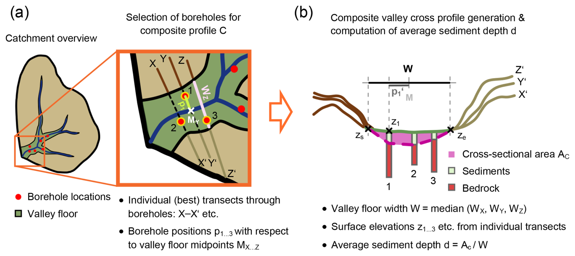
Figure A1 Details of valley cross sections in addition to Fig. 2 and Sect. 4.2. Panel (a) exemplarily shows the best transects through selected boreholes within a catchment section. Panel (b) displays the valley cross section composed of these boreholes, including respective sediment depths, positions across the valley, and relevant surface elevations z from the individual transects.

The average sediment depth d of a composite cross profile is computed by dividing the cross-sectional area A_c of the sedimentary infill of a valley through the valley floor width W (Eq. 1, Sect. 4.2). Therefore, A_c is approximated by linear interpolation, i.e., a segmentation into several sections consisting of triangular areas towards the valley floor border and of trapezoidal areas between the single boreholes. Thereby, z_s and z_e each refer to the valley floor border surface elevations of the individual transects of both boreholes closest to the rim of the valley (Fig. A1). Moreover, borehole surface elevations $z_{\mathrm{1},\mathrm{\dots },n}$ for n boreholes in the composite cross profile, as well as the associated sediment depths and a linear interpolation, were utilized to create the assumed cross-sectional area.

Moreover, the direction and position, respectively, of the composite profiles as indicated in the maps Figs. 3 and S1 in the Supplement are defined as the direction of the central individual transect (see Fig. A1a; here: transect Y–Y^′) and the center between the valley midpoints of both outermost individual transects (here: transects X–X^′ and Z–Z^′). Therefore, all transects within a composite profile are sorted by the coordinates of their valley floor midpoints M in the SW–NE, W–E, or NW–SE direction.

Appendix B

In order to produce grids of flow value accumulation across the valley floor, for every grid cell c[i, j] within the valley floor, transects through that cell and across the valley floor in four directions (N–S, NE–SW, E–W, SE–NW) were constructed (Fig. B1); this relatively simple approach was chosen to keep computing time at a low level. The cell's associated maximum flow accumulation value was then drawn from the maximum of the shortest of these transects across the valley, assumed to represent the most direct path, and of both adjacent transects. The latter was crucial to catch the maximum values also in the case of diagonal transects or channels at the rim of the valley bottom.

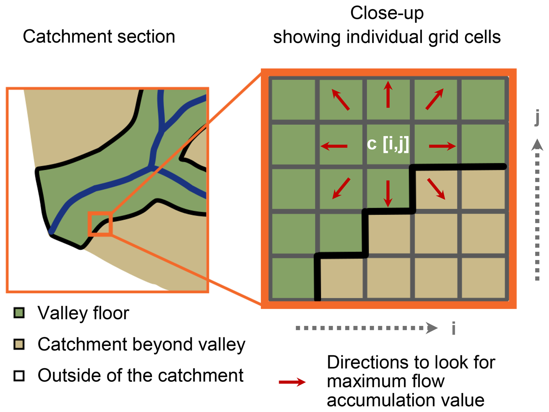
Figure B1 Details of the grid-based computation of flow value accumulation across the valley floor.

To smooth values, a median filter was applied to the resulting grid twice: for all cells c[i, j] within the valley floor, a new grid with

$$\begin{array}{}\text{(B1)}& c[i,j{]}^{\ast }=\mathrm{med}\left(c\left[i+k,j+k\right]\right),\end{array}$$

with $k\in \mathit{\{}-\mathrm{1},\mathrm{1}\mathit{\}}$ neglecting NA values, was created; i.e., a cell's value was replaced by the median of its eight adjacent cells.

Moreover, visual inspection of preliminary results showed geometry-related edge effects at the catchment outlets with values decreasing again. To prevent these artifacts, grid cells at the downstream edge of the valley floor were simply set to the catchment's flow accumulation maximum. The affected grid cells were defined based on the elevation quantile of the grid cell of the flow accumulation maximum, plus a buffer (0.002 for all catchments, except 0.01 for the Dreisam and 0.11 for the Neumagen) that was individually adjusted so that valley floors of incoming tributaries were not affected.