A composite ¹⁰Be, IR-50 and ¹⁴C chronology of the pre-Last Glacial Maximum (LGM) full ice extent of the western Patagonian Ice Sheet on the Isla de Chiloé, south Chile (42° S)

Unanswered questions about the glacier and climate history preceding the global Last Glacial Maximum (LGM) in the southern temperate latitudes remain. The Marine Isotope Stage (MIS) 3 is normally understood as a global interstadial period; nonetheless its climate was punctuated by conspicuous variability, and its signature has not been resolved beyond the polar realms. In this paper, we compile a ¹⁰Be depth profile, single grain infrared (IR) stimulated luminescence dating and ¹⁴C samples to derive a new glacier record for the principal outwash plain complex, deposited by the western Patagonian Ice Sheet (PIS) during the last glacial period (Llanquihue Glaciation) on the Isla de Chiloé, southern Chile (42^∘ S). In this region, the Golfo de Corcovado Ice Lobe left a distinct geomorphic and stratigraphic imprint, suitable for reconstructing former ice dynamics and timing of past climate change. Our data indicate that maximum glaciation occurred by 57.8±4.7 ka without reaching the Pacific Ocean coast. Ice readavanced and buttressed against the eastern side of the Cordillera de la Costa again by 26.0±2.9 ka. Our data further support the notion of a large ice extent during parts of the MIS 3 in Patagonia and New Zealand but appear to contradict near contemporaneous interstadial evidence in the southern midlatitudes, including Chiloé. We propose that the PIS expanded to its full-glacial Llanquihue moraines, recording a rapid response of southern mountain glaciers to the millennial-scale climate stadials that punctuated the MIS 3 at the poles and elsewhere.

1 Introduction

We lack thorough knowledge on the timing of the local Last Glacial Maximum (lLGM) for the Southern Hemisphere mountain glaciers because the dating of their terminal moraines and associated outwash plains has remained spatially variable. Understanding the glacial fluctuations throughout this recent glacial period (e.g., Marine Isotope Stage, MIS, 4 through MIS 2) is a prerequisite for uncovering the cause and climate mechanisms driving southern glaciation and the interhemispheric linkages of climate change (Denton et al., 1999a). Similarly, defining the ice extent is key for understanding the magnitude of the last glaciation in the southern Andes (e.g., the lLGM) and thereby the main paleoclimatological, geomorphological and paleoecological implications. In addition to MIS 2, new records indicate extensive glaciers during MIS 3, MIS 4 and late MIS 5 in southern Patagonia and New Zealand, but uncertainty remains as to whether this is a common feature of southern midlatitude glacial history (Schaefer et al., 2015; Williams et al., 2015; Darvill et al., 2015; Kelley et al., 2014; García et al., 2018; Davies et al., 2020; Mendelová et al., 2020; Shulmeister et al., 2010). Moreover, the MIS 3 is normally referred to as a global interstadial period when southern conifer forest expanded to ice-free low-land areas, but glaciers are also known to have advanced in southern Chile and New Zealand by this time (Villagrán et al., 2004; Kelley et al., 2014; Darvill et al., 2015; García et al., 2018). Despite the fact that paleoclimate records are well-resolved in the polar regions, main knowledge gaps remain for the terrestrial southern midlatitudes before the global LGM time frame.

Here, we present new geochronological data from a ¹⁰Be depth profile, infrared (IR) stimulated luminescence dating using single grains of potassium-rich feldspar (Fs) and ¹⁴C samples of the two Cucao main outwash terraces (Cucao_T1 and Cucao_T2) on the Isla de Chiloé, south Chile (42^∘ S) (Figs. 1 and 2). These extensive outwash plains were deposited by the Golfo de Corcovado Ice Lobe of the northwest Patagonian Ice Sheet (PIS) during the Llanquihue Glaciation (i.e., the last glacial period). Together with Cucao_T1 and Cucao_T2, multiple pairs of outwash terraces occupying similar morphostratigraphic positions occur on the lee side of the Cordillera de la Costa and represent the full glacial extent in Chiloé (Fig. 1). These outwash terraces can be traced to ice-contact slopes on the east side of the Cordillera de la Costa as they have been previously mapped (García, 2012). Thus, the dating of the Cucao_T1 and Cucao_T2 terraces can help reconstruct the lLGM of the PIS and the overall glacier and climate history that preceded the well-known LGM (MIS 2) in the region (Mercer, 1976; Laugénie, 1982; Porter, 1981; Bentley, 1997; Denton et al., 1999b). Our record builds on previous work in the Chilean Lake District (CLD) by dating glacially derived sediments that can be directly related to a landform, thereby determining the extent of glacier advances during the last glacial period. Dating landforms beyond the ¹⁴C range in Chiloé is challenging. Exposed bedrock and boulders resting on glacial landforms are very rare, rendering commonly used cosmogenic nuclide exposure-dating techniques impractical. Here, we constrain the timing of maximum ice extent, as recorded by glacial landform and deposit associations, by applying a composite geochronologic approach.

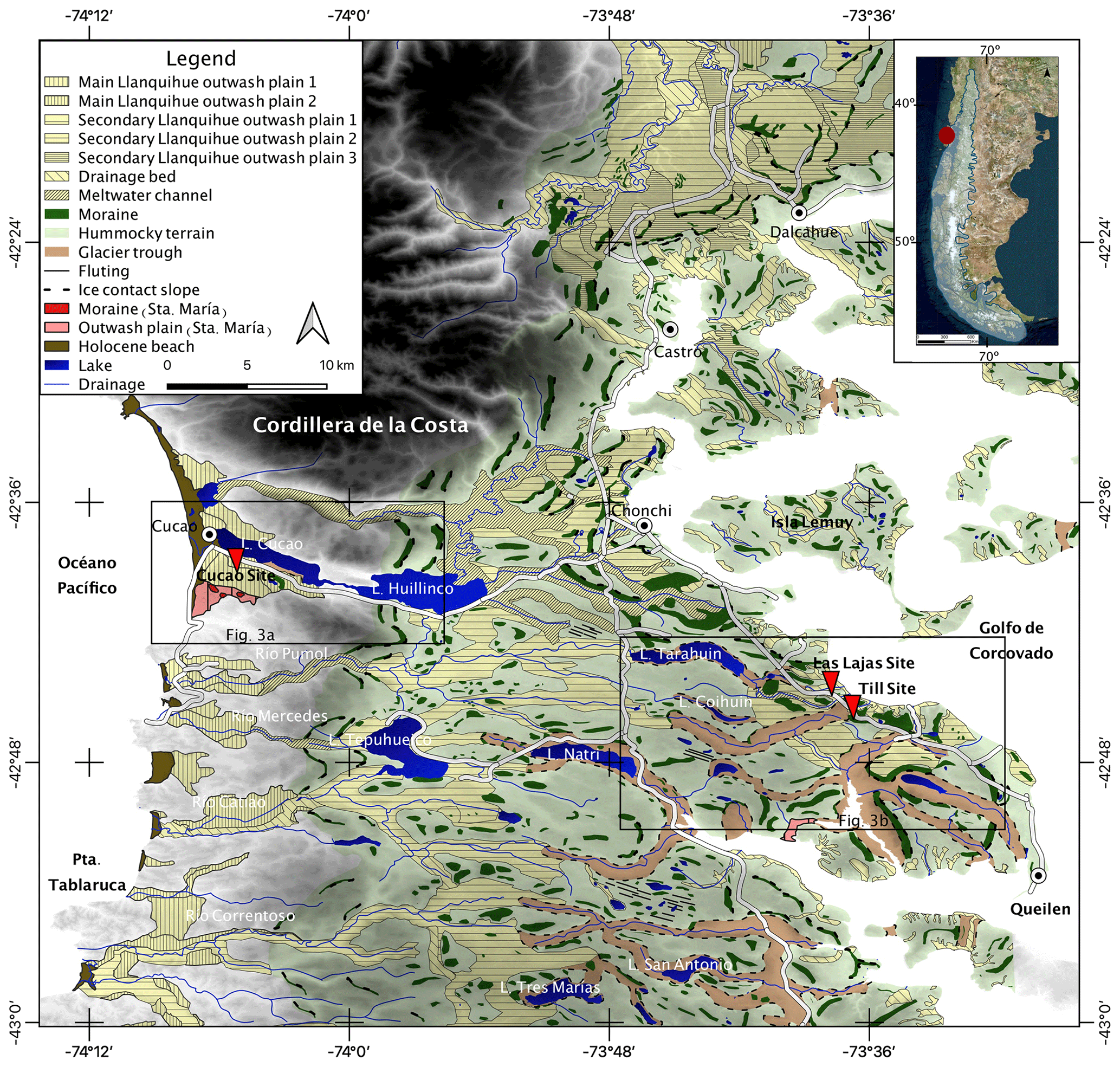
Figure 1 The Cucao site in the context of the former Patagonian Ice Sheet (PIS) and the glacial geomorphologic setting of the Archipiélago de Chiloé. The red circle in the inset indicates the location of the study area in the northwest sector of the former PIS (outlined). Note the location of stratigraphic sites presented in this study and mentioned in the text. For the sake of space, the Cucao site in the map indicates the geographic location of all seven sites studied within this sector. For more details, see Figs. 2 and 3a. Geomorphic map modified from García (2012). Base map is the 30×30 Shuttle Radar Topography Mission (SRTM) extracted from NASA JPL (2013).

Figure 2 Oblique view of the Cucao_T1 and Cucao_T2 outwash terraces and the studied Cucao sites. All Cucao sites occur in these terraces on the western side of the Cordillera de la Costa. View is to the south-southeast. Ice flow from the upper left. Base image from © Google Earth.

1.1 The Llanquihue Glaciation

The Llanquihue Glaciation is the local name for the last glacial period in southern Chile, particularly the CLD and the Archipiélago de Chiloé (39–42^∘ S) (Heusser and Flint, 1977; Porter, 1981; Laugénie, 1982; Denton et al., 1999b; García, 2012). Glacial landforms and sediments from the last ice period display excellent preservation and limited weathering, respectively. García (2012) suggested that a mountain style of glaciation characterized the CLD. Different subglacial landforms, including drumlinoid and fluting landforms, within extensive, mostly uninterrupted ice-marginal positions denote rather an ice-sheet style of glaciation to the south on the Isla Grande de Chiloé. For instance, a west–east transect across the moraine field in the CLD and northern Isla de Chiloé reveals a stepwise topography punctuated by distinct ice-contact slopes, composite moraines, and associated main and subsidiary outwash plains (Andersen et al., 1999; Denton et al., 1999b). To the south of Dalcahue, a double moraine and ice-contact slope preserved on the eastern slope of the Cordillera de la Costa represents the outermost extents of the ice during the Llanquihue Glaciation in Chiloé (García, 2012). Beyond this ice-marginal position, meltwater channels carved the bedrock and fed outwash terraces on the Pacific mountain side. Accordingly, the Huillinco and Cucao lakes (Fig. 1), which interrupt the continuity of the Cordillera de la Costa, likely allowed the ice to trespass towards the west. Otherwise, the ice buttressed on the eastern mountain side. It has been suggested that the outer Llanquihue landforms (i.e., the early Llanquihue time) were deposited during the Marine Isotope Stage (MIS) 4 (e.g., Denton et al., 1999b; García, 2012). This conclusion is based on the landform and sediment preservation, together with the infinite uncalibrated age >50 000 ¹⁴C yr BP, of the Taiquemó record (Heusser et al., 1999), which is located inboard from the early Llanquihue moraine in northern Chiloé. In addition, sea surface temperatures (SSTs) offshore northern Chiloé uncover the coldest glacial conditions in the ocean during MIS 4 (Kaiser et al., 2005). Nonetheless, the early Llanquihue landforms have remained mostly undated, which in turn is the main research focus of this paper.

The MIS 3 in Chiloé and the CLD have been regarded as an interstadial period based on pollen and sub-fossil-tree records constrained by finite and mostly infinite ¹⁴C ages (e.g., Heusser et al., 1999; Roig et al., 2001; Villagrán et al., 2004). At this time conifer forests dominated, indicating a relatively mild and humid climate (Villagrán et al., 2004). However, high variability between arboreal and herbaceous vegetation also occurred, which suggests climate instability through the MIS 3 (Heusser et al., 1999). The same conclusion can be extracted from the SST record offshore Chiloé (Kaiser et al., 2005).

For MIS 2, Denton et al. (1999b) determined the timing of at least four glacial advances in the CLD and northern Isla Grande de Chiloé, which significantly added to the previous work in the region (Mercer, 1976; Porter, 1981; Bentley, 1997). From their radiocarbon chronology, Denton et al. (1999b) defined the timing of the LGM to between 34.3 and 18.0 cal kyr BP. In central Chiloé, a glacial advance occurred before 28 cal kyr BP and at 26.0 cal kyr BP (García, 2012). The regional equilibrium line altitude (ELA) was depressed ∼1000 m relative to the present (Porter, 1981; Hubbard et al., 2005). This corresponds to an estimated drop of 6 to 8 ^∘C in mean summer temperature and mean annual precipitation ∼2000 mm yr⁻¹ greater than present (Heusser et al., 1996, 1999; Villagrán, 1988, 1990). The end of the LGM was marked by abrupt glacial retreat after 18 cal kyr BP, both in the CLD and Chiloé (Lowell et al., 1995; Denton et al., 1999b).

1.2 Regional setting

The Archipiélago de Chiloé is separated from the mainland by the Golfo de Ancud and Golfo de Corcovado, where intervening seawaters can reach >400 m but mostly less than 200 m depth. The western Patagonian Andes facing Chiloé reach higher elevations and contain a significantly larger number of glaciers than the CLD to the north, with ice caps on peaks >2000 m a.s.l. (Barcaza et al., 2017).

South of 40^∘ S, the southwesterly circulation is present throughout the year (Garreaud et al., 2009). This zonal wind extends through the whole troposphere and occurs as a mostly symmetric belt in the southern midlatitudes. The westerly wind belt in the Pacific occurs in a zone constrained mainly by the effect of the subtropical anticyclone and the polar front, and today it produces a precipitation peak at 45–47^∘ S (Miller, 1976). Seasonal expansion (winter) and contraction (summer) of the westerly wind belt and associated storm circulation govern the climate along extratropical Chile. Chiloé intersects the northern margin of the westerly wind belt, which results in humid winters (>1000 mm of precipitation between May–August in Castro; Luebert and Pliscoff, 2006) and rather dry summers due to the blocking effect of the Pacific high-pressure cell (Miller, 1976; Garreaud et al., 2009). In South America, precipitation to the west of the southern Andes chain is positively correlated to the westerly wind strength, while the opposite occurs to the east of the Andes, where a rain shadow dominates (Garreaud, 2007). Mean air temperatures in Chiloé fluctuate from about 8 ^∘C in winter to 14 ^∘C in summer, reflecting a west-coast, southern-midlatitude maritime climate regime. Nonetheless, freezing temperatures can occur late in the autumn. Climate variability at decadal to interdecadal timescales is affected by pressure anomalies in the Antarctic and the southern midlatitudes (the Southern Annular Mode, SAM) thus controlling the strength and position of the westerly wind, precipitation yields and surface air temperatures south of 40^∘ S (Garreaud et al., 2009, 2013).

Offshore Chiloé, the north branch of the Antarctic Circumpolar Current (ACC) shows the steepest thermal latitudinal gradient (Kaiser et al., 2005). This abrupt change in SST temperatures is linked with the southwesterly wind's northern boundary (Strub et al., 1998). Just south of Chiloé, the ACC separates into the northward Humboldt Current and the southward Cape Horn Current (Lamy et al., 2015). The Humboldt Current transports subantarctic surface waters of the ACC along the Chilean coast with mean annual SST offshore Chiloé reaching ∼13 ^∘C (Kaiser et al., 2005). The ocean and atmosphere circulation are intimately linked and experienced large changes during the LGM affecting the PIS fluctuations (Lamy et al., 2015).

2 Methods

For studying the Cucao terraces, we selected a total of seven sites, including sediment pits and road sediment sections in both Cucao_T1 and Cucao_T2 (Figs. 2 and 3a). The number and distribution of sites help us to constrain the age of these glaciofluvial landforms. Most of sites occur on top of the glaciofluvial plains (sites Cucao_T1_1–3 and _7) except for Site Cucao_T1_4, Site Cucao_T2_5 and Site Cucao_T2_6, which occur by the edge of the terraces. We also study a stratigraphic section in eastern Chiloé (the Till site) which, together with the Las Lajas site (García, 2012), adds context for interpreting Cucao data.

Figure 3 Geomorphic maps showing the morphostratigraphic relationships between the Cucao sites (a) and Las Lajas and Till sites (b). Also shown in (a) are the inferred ice limits (dashed lines) associated with the deposition of Cucao_T1 and Cucao_T2 terraces. Both of these terraces are separated by a distinct fluvial scarp that in part could have been formed as an ice contact slope (see text for discussion). Legend codes in Fig. 1.

2.1 Mapping and sedimentology

The mapping produced here builds on previous work in the area (Heusser and Flint, 1977; Andersen et al., 1999; García, 2012). We took advantage of new sediment exposures in the study area to produce more detailed observations of sediments and landforms during multiple field campaigns developed between 2016–2019. For better description and interpretation of the geomorphology, we analyzed SRTM_GL1 (Nasa JPL, 2013) and reexamined aerial photographs of the study area. Sediment analysis includes modified facies codes based on Miall (1985, 2006), Eyles et al. (1983), and Maizels (1993). We applied traditional sedimentology and geomorphology techniques in order to describe the glacial and proglacial environments as a basis for our dating approach.

2.2 Geochronology

2.2.1 Radiocarbon

We radiocarbon dated both bulk organic sediment and wood samples. We targeted in situ organic stratigraphic units or reworked organic mud clasts embedded in outwash sediments. The interpretation of our ¹⁴C data varied depending on the setting, as described in the results section. All ¹⁴C ages in this paper are presented as the mean ± uncertainty of the reported 2σ range except where indicated. The ages were calculated using CALIB REV7.1 online web calculator (Stuiver et al., 2020) and the Southern Hemisphere ¹⁴C calibration curve (Hogg et al., 2013). The ¹⁴C calibrated ages include >0.9 probability within the 2σ range. This is true for all data presented except sample CUCAOT1-1803_III (>0.7).

2.2.2 The ¹⁰Be depth profile

We selected a stratigraphic column at the Site Cucao_T1_3 section with an accessible sediment depth reaching ∼300 cm (Fig. 4). This site is suitable for building a ¹⁰Be depth profile as the sediments appear to have been deposited on top of each other in a continuous and rapid fashion (Hein et al., 2009; Darvill et al., 2015). Nonetheless, the sediment section where the ¹⁰Be profile was sampled includes a top organic soil (upper 35–20 cm) that overlies outwash sediment, and therefore no surface cobbles were found for dating. An iron-rich layer occurs at 70 cm below the original surface within the outwash sediments. Above this iron layer, the sediment can appear oxidized, which is not the case towards the bottom of the sediment section.

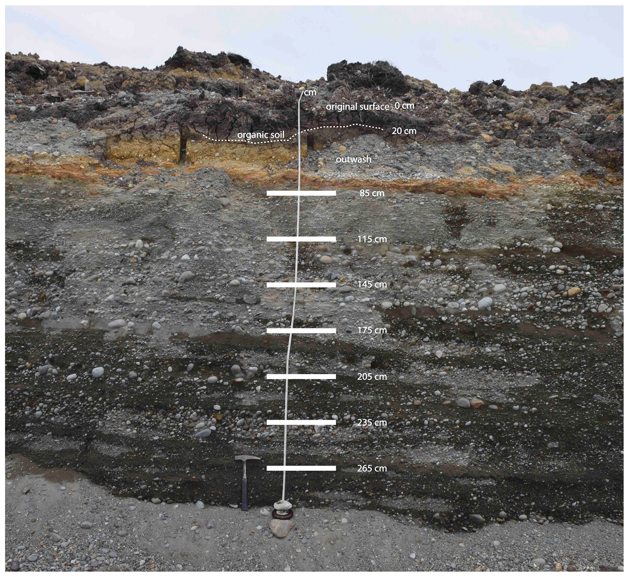
Figure 4 Cucao_T1 ¹⁰Be depth profile produced in Cucao_T1_3 site. Note the original surface (underlying not in situ mixed soil remains) and the in situ organic soil and outwash sediment surface contact (dashed white line). Solid white rectangles indicate ¹⁰Be sample locations with associated depths.

The most critical parameter to model how the ¹⁰Be accumulates underground is the evolution of the surface erosion/accretion affecting the depth of the quartz grains (samples) through time. This is because the cosmogenic ¹⁰Be production rate decreases exponentially with cumulative mass depth (expressed in g cm⁻²). To relate cumulative mass depth to the sampling depth within a sediment layer requires an estimate of the overlying bulk soil density. For our model, we considered the outwash sediment bulk density to be between 1.9 and 2.2 g cm⁻³, based on the visual estimation of porosity between 20 % and 30 %, with variable moisture between 30 % and 60 %, and for a grain density of 2.6 g cm⁻³. This density range coincides with the densities of gravel-bearing unconsolidated materials listed in Manger (1963). We include the top organic soil (see Sect. 3) in this range. For testing our ¹⁰Be profile models for Cucao_T1_terrace, ¹⁰Be concentrations produced in situ were measured in quartz obtained from seven amalgamated sand and pebble sample layers. We collected about 3 cm thick layers each 30 cm between 85–265 cm depth (Fig. 4). Model concentrations were calculated at the center of the sampling layers. We did not sample the top 50 cm of the outwash to avoid vertical sediment mixing due to potential root development near the surface.

Sediment ¹⁰Be sample preparation as an accelerator mass spectrometry (AMS) target was done at University of Edinburgh's cosmogenic nuclide laboratory. The ¹⁰Be was selectively extracted from 20 to 26 g of pure quartz following standard methods (Bierman et al., 2002; Kohl and Nishiizumi, 1992). The samples and the process blanks (n=1) were spiked with ∼0.25 mg ⁹Be carrier (Scharlau Be carrier, 1000 mg L⁻¹, density 1.02 g mL⁻¹). The samples were prepared as BeO targets for AMS analysis following procedures detailed by Hein (2009). Measurements of ${}^{\mathrm{10}}\mathrm{Be}{/}^{\mathrm{9}}\mathrm{Be}$ ratios were undertaken at CologneAMS (Dewald et al., 2013), normalized to the revised standard values reported by Nishiizumi et al. (2007). Blank ${}^{\mathrm{10}}\mathrm{Be}{/}^{\mathrm{9}}\mathrm{Be}$ ratios ranged between 1 % and 5 % of sample ${}^{\mathrm{10}}\mathrm{Be}{/}^{\mathrm{9}}\mathrm{Be}$ ratios. Table 1 shows other ¹⁰Be data from this study.

Table 1 The ¹⁰Be data for depth profiles in the Cucao_T1 terrace.

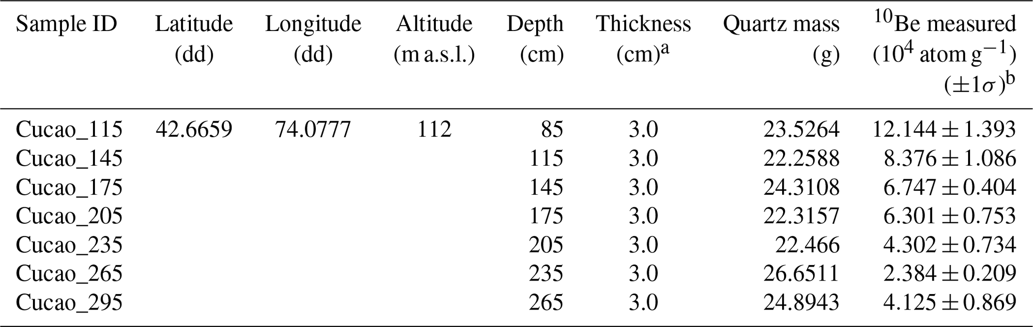
^a This is the approximate thickness of the layer of amalgamated sediment collected at each specified depth. ^b Nuclide concentrations are normalized to revised ¹⁰Be standards and half-life (1.36±0.07 Myr) of Nishiizumi et al. (2007) and include propagated AMS sample and lab-blank uncertainty and 2 % carrier mass uncertainty. Quartz density is 2.7 g cm⁻³. Topographic shielding at the profile site is negligible (0.9999).

The ¹⁰Be accumulation was modeled following the formulae of Lal (1991). The time was discretized to accommodate the change in the samples' depths due to the accumulation of the overlaying organic sediment. Monte-Carlo simulations (as in Hidy et al., 2010) were used to find the fitting values of the following free parameters: (1) the age of the outwash sedimentary package, (2) the age of the overlaying organic soil and (3) the initial ¹⁰Be accumulated before the outwash deposition, which is considered to be constant along the outwash profile. Random values of bulk density between 1.9 and 2.2 g cm⁻³ were considered for the entire profile. Probabilities corresponding to the chi-square values of the individual models were used to calculate the probability density distributions of the parameters. The method described in Rodés et al. (2011) was used to select the models fitting the data within a 1σ confidence level. We initially modeled the effect of gradual (linear with time) accretion of the organic sediment. The Be-10 profiles under the organic sediment generated by these models were identical to those generated for instantaneous deposition of the organic sediment layer at an intermediate time (between the outwash formation and today). Therefore, the formation age of the organic sediment was considered an unknown variable in the models presented here in order to simulate all extreme scenarios. As the timing of the process that produced the organic soil is unknown, two scenarios were considered. Scenario “a” does not consider the shielding produced by the organic layer, as would be appropriate if the latter was formed recently or for a limited time span. The models fitting this scenario provide a minimum estimate for the outwash deposition age as they consider the conditions that maximize the ¹⁰Be production rate at the sample depths. Scenario “b” considers that the organic layer could be deposited anytime between the outwash deposition and today. The models fitting this scenario should cover all the possible and the less restrictive age ranges for the deposition of the Cucao_T1 outwash. The models assume no surface erosion occurred after outwash deposition as negligible erosion rates are expected in abandoned outwash plains in relatively short time spans (i.e., the last glacial period) (Hein et al., 2009). We used ¹⁰Be production rates of 4.0678, 0.0383 and 0.0404 atoms g⁻¹ and attenuation lengths of 160, 2481 and 1349 g cm⁻², for spallation and fast and stopping muons, respectively. This is in agreement with the average production rate corresponding to the Lago Argentino calibration data in Patagonia (Kaplan et al., 2011) scaled according to the online calculators formerly known as the CRONUS-Earth online calculators v.3 (Balco et al., 2008) for the last ∼100 kyr and using the scaling scheme of LSDn (Lifton et al., 2014). The LSDn is based on models derived from theory and includes estimates for a time-dependent magnetic field (Lifton et al., 2014). Although the selection of this scaling scheme does not affect our conclusions, we chose to use the Lago Argentino calibration and LSDn scaling scheme in order to facilitate the direct comparison of our ages with other published cosmogenic ages in Patagonia (e.g., Davies et al., 2020).

2.2.3 Luminescence dating approach

We collected luminescence samples by driving opaque tubes into soft sand sediments within the outwash deposits of Cucao_T1 (sites _1, _2 and _3; four samples) and Cucao_T2 (sites _5 and _6; two samples). Luminescence dating techniques in general allow for the determination of depositional ages of sediments by calculating the point in time when the sediments were last exposed to daylight (during transport) and subsequently shielded from daylight (deposition). The build-up of a latent luminescence signal in quartz- and potassium-rich feldspar minerals is time dependent and induced by naturally occurring radiation (cosmic radiation and ionizing radiation from naturally occurring radionuclides). Once the stored luminescence signal (termed equivalent dose) and the rate of ionizing radiation impacting the sample over time (termed the dose rate) are known, a luminescence age can be determined using the following general age equation: age (a) = equivalent dose (Gy) $/$ dose rate (Gy a⁻¹). For further details on luminescence dating in general, please see the following overview papers: Preusser et al. (2008), Rhodes (2011), Wintle (2008), and Smedley et al. (2016).

All sample preparation and subsequent measurements were conducted at the Vienna Laboratory for Luminescence dating (VLL) on RISØ DA20 luminescence reader systems, one of which is equipped with an 830 nm infrared laser for the stimulation of the luminescence signal of potassium-rich feldspar single grains (Bøtter-Jensen et al., 2000, 2003). All measurements were conducted using potassium-rich feldspar because quartz from Patagonia has frequently been shown to be unsuitable for dating purposes (García et al.,  2019; Duller, 2006; Glasser et al., 2006; Harrison et al., 2008; Blomdin et al., 2012; Smedley et al., 2016). All sample preparation was conducted at the VLL under subdued red light conditions to extract pure separates of potassium-rich feldspar (procedures described in detail in Lüthgens et al., 2017). Because water-lain samples in general are prone to incomplete bleaching of the luminescence signal prior to burial (insufficient exposure to daylight to reset the luminescence signal to zero), and that effect is intensified by the slow bleaching properties of potassium-rich feldspar, a single grain dating approach was adopted to detect and correct for the effects of incomplete bleaching. This methodological approach has been described in detail in García et al. (2019). All measurements were conducted using an IR-50 (infrared stimulated luminescence at a temperature of 50 ^∘C) SAR (single aliquot regenerative) dose protocol, using the most easily bleachable K-feldspar (potassium-rich feldspar) signal (Blomdin et al., 2012). Rejection criteria (<30 % recycling ratio, <30 % recuperation, <20 % test dose error) are based on results from dose recovery experiments resulting in recovery ratios in agreement with unity within error. Equivalent dose values were calculated using the bootstrapped three-parameter minimum age model (BS-MAM; Galbraith et al., 1999; Cunningham and Wallinga, 2012) with a threshold value of 40±10 % for the expected overdispersion. The threshold value is based on the results from dose recovery experiments and the characteristics of the best-bleached natural sample (Figs. 5 and 6). All statistical evaluation was done using the R luminescence package of Kreutzer et al. (2012). The contents of naturally occurring radionuclides (²³⁸U and ²³²Th decay chains, as well as ⁴⁰K) contributing to the external dose rate were determined using high-resolution, low-level gamma spectrometry (Baltic Scientific Instruments 40 % p-type HPGe detector). The dose-rate and age calculation was conducted using the software ADELE (Kulig, 2005), and all ages were corrected for fading (athermal signal loss over time; Wintle, 1973) using the approach of Huntley and Lamothe (2001) based on an average fading rate (g value of 4.4±0.27) from multiple samples determined following the approach of Auclair et al. (2003) on multi-grain aliquots, as suggested by Blomdin et al. (2012). All details concerning the experimental setup are described in García et al. (2019) and the supplement on luminescence dating in that paper. A typical dose response curve and a typical equivalent dose distribution are provided in Figs. 5 and 6 for sample VLL-0291-L. In the text, we provide the calculated IR-50 age ± 1σ.

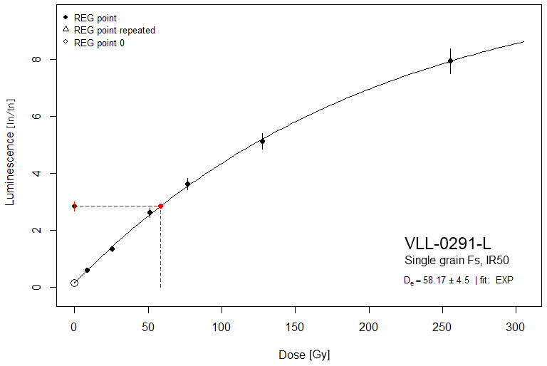
Figure 5 Representative dose response curve for a single K-feldspar grain of sample VLL-0291-L. Plot generated using the R luminescence package of Kreutzer et al. (2012).

Figure 6 Equivalent dose distribution for sample VLL-0291-L. KDE plot (kernel density estimate) generated using the R luminescence package of Kreutzer et al. (2012). The graph shows an asymmetric, right-skewed distribution, which is typical for incompletely bleached samples.

3 Results

Whereas the higher Cucao_T1 outwash plain occurs at ∼140 m a.s.l., the lower Cucao_T2 occurs at ∼70 m a.s.l. Nonetheless, both landforms show relatively high topographic gradients between ∼2 % (Cucao_T1) and ∼1.3 % (Cucao_T2). Multiple outwash levels exist in between these two large outwash plains, but they are only local in extent. A main geomorphic feature is a ∼30 m tall scarp that separates Cucao_T1 and Cucao_T2 terraces (Fig. 3a). To the west, the Cucao_T2 terrace is punctuated by a hummocky terrain adjacent to the T1 terrace scarp where the Quilque lake develops (Fig. 3a). The most prominent mounds are covered by dense forests, but a recently cleared inner ridge exhibits a diamictic surface with several rounded cobbles and small boulders on top partly covered by soil development. Overall, these landforms resemble a type of moraine relief surrounded by Cucao_T2 outwash plain. The links between this moraine landform and the outwash terraces are discussed below in Sect. 4.

3.1 Sedimentology

We selected a total of six sites for stratigraphic sediment interpretation: Cucao_T1 is characterized by the description of sites _1–_4. Cucao_T2 is characterized based on sites _5 and _6 (see Figs. 2 and 3a for location and Table 2 for site details). Sedimentological description and interpretation provided here for Cucao_T1 and Cucao_T2 terraces allow us to discuss the type of glacial and proglacial setting during maximum glaciation in Chiloé. Site Cucao_T1_7 outcrops on the side of a road as a nearly 50 cm peat deposit, and therefore no sediment description was made here.

Table 2 Sediment sections analyzed in this study.

^* García (2012).

3.1.1 Site Cucao_T1_1

The exposure consists of a series of crudely bedded, well-rounded, clast- to matrix-supported gravels (Gmg, Gcg), arranged in 0.3–0.5 m subhorizontal beds (Fig. 7a). Predominant grain size is within the pebble range, although cobble-rich bodies are common. Both upward-coarsening and upward-finning beds occur, matrix content generally decreasing from base to top and usually culminating in a clast-supported veneer. Beds are laterally extensive (>10 m) and mostly bounded by flat subhorizontal surfaces occasionally disrupted by shallow, narrow channel bodies filled with matrix-supported, massive, cobble-rich, imbricated gravels (Gmm, Gmi). Polymict material is predominantly of Andean origin (volcanic and intrusive rocks).

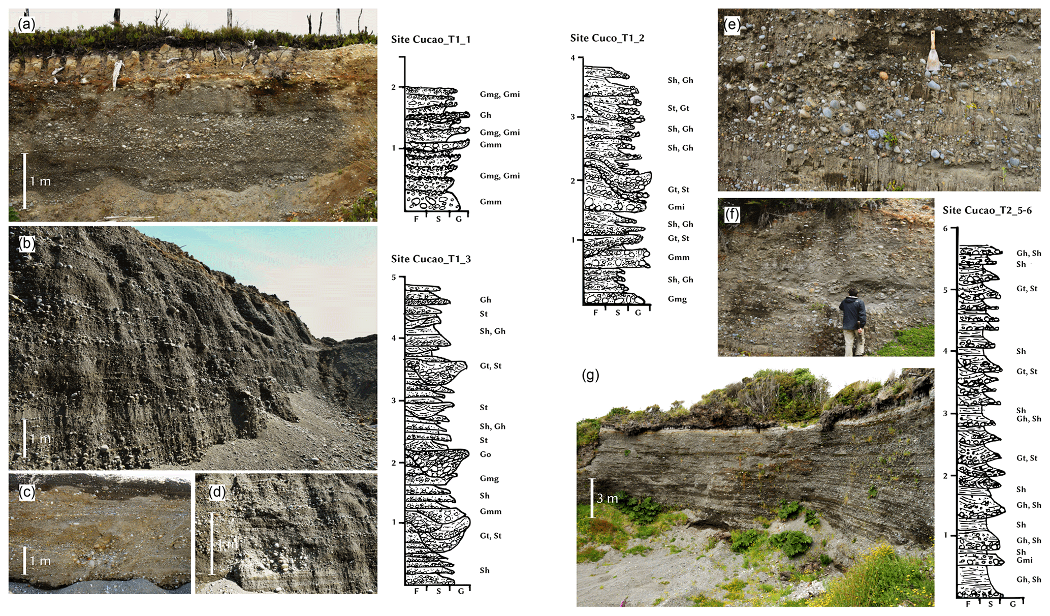
Figure 7 Generalized stratigraphic columns and sedimentary attributes for studied sites within Cucao terraces. (a) Cucao_T1_1, laterally extensive gravel beds, mostly bounded by flat subhorizontal surfaces but occasionally filling shallow channel-shaped depressions. (b) Cucao_T1_3 wide view. Note pebble to small cobble layer at the base of most lower bounding surfaces. (c, d) Detail of small channel bodies within Cucao_T1_3. Images come from two opposing walls about 3 m apart and capture the same channel element: a small open-framework gravel-filled (Go) channel in (d) grading downflow to a wider multistory filled channel in (c). This is interpreted as an entrenched gully. (e, f) Cucao_T1_2: (f) shows a general view capturing one of the channel-shaped bodies referred to in the description, while (e) shows a detail of stacked gravel and sand layers that characterize this exposure. (g) Cucao_T2_5–6, general view of sediments in Site 6. Because of similarities between both sites (5 and 6) we only show a single column that represents Cucao_T2 sediments.

Interpretation. Gcg and Gmg are interpreted as being the product of turbulent and cohesive debris flows, respectively. Laterally extensive beds, making up most of the exposed sequence, are interpreted as being the result of unconfined sheet floods. Most beds are capped by a clast-supported veneer inferred to represent winnowed sediments. Shallow channel bodies filled by Gmm and Gmi facies are taken to indicate, respectively, cohesive and turbulent, channelized, possibly erosive debris flow deposits. The whole section would thus be composed of gravitationally resedimented glacial sediments chiefly through the action of both channelized and unchannelized debris flows.

3.1.2 Site Cucao_T1_2

This is a road cut exhibiting a series of rounded, poorly to moderately sorted, matrix- to clast-supported gravel and sand layers disposed in ∼ 0.1–0.3 m thick subhorizontal beds (Fig. 7e–f). Gravel is mostly within the range of pebbles. Crudely bedded, matrix-supported, chaotic and usually coarsening upwards beds (Gmm, Gmg) form laterally extensive lenses. Clast- to matrix-supported, crudely bedded and imbricated gravel layers (Gmi, Gh) alternate with parallel-stratified, pebbly sand layers (Sh) forming a series of fining upwards sequences. Lateral extension is often truncated by concave-upwards basal surfaces of channel-shaped bodies up to 0.9–1.2 m deep filled with similar sediments. Within these fills, festoon patterns are common (St, Gt). A few outsized muddy intraclasts occur throughout the exposure.

Interpretation. Gmm and Gmg facies are interpreted as cohesive through turbulent debris flow deposits. Gmi, Gh and Sh are related to traction deposits under waning flow conditions associated with periodical shifts in hydraulic regime. Channel bodies' frequently truncating strata are taken as the product of a highly unstable, rapidly shifting distributary system made up of narrow, shallow channels.

3.1.3 Site Cucao_T1_3

This is a gravel pit, 8 m deep at most and topped by an organic soil unit (Fig. 7b–d). Exposure here consists of a series of poorly to moderately sorted, well-rounded, clast- to matrix-supported gravel and sand layers. Beds are between 0.1 and 0.4 m thick and several meters wide, with sharp subhorizontal or concave-upwards bounding surfaces often cutting underlying stratification at low angles. Both upward coarsening and upward fining layers occur, though the latter is more common. Beds usually show crude horizontal stratification (Gh, Sh) and trough or tabular cross-bedding (Gt–Gp, St–Sp). Small scours ∼0.9 m wide and ∼0.5 m deep filled with clast-supported, open-framework large pebbles to small cobbles (Go) are present as isolated features or within larger, 2–3 m wide and ∼1.5 m deep multistory channels. Matrix-supported, chaotic gravels (Gmm) occur almost exclusively within these fills. A few outsized, rounded, mud intraclasts lie within Sh and Gh facies.

Interpretation. Facies Gh, Gt–Gp, Sh and St–Sp are consistent with deposition from traction load within streamflows. Gmm facies are interpreted as debris flow deposits. Low-angle cutting is inferred to represent reactivation surfaces, reflecting a change in hydrological conditions between series of stacked traction carpets (i.e., third order surfaces in Miall, 2006). Wider multistory channel elements would represent entrenched channels active during low water stages. Altogether, deposits suggest an environment with a highly variable discharge that is prone to periodical flooding and channel instability. The whole sequence is here inferred to represent deposition within a shallow braided distributary system, with a minor contribution – or low preservation – of debris flows. The presence of mud intraclast can suggest incipient soil development within interfluves.

3.1.4 Site Cucao_T1_4

This consists of clast-supported, poorly to moderately sorted, trough cross-bedded gravel and sand (Gt, St) (Fig. 8). They are arranged in 0.5–1 m deep and >3 m wide channel-shaped bodies. Towards the terrace edge, an inclined erosion surface cuts through all strata and is mantled by a chaotic to crudely bedded diamicton (Dmm).

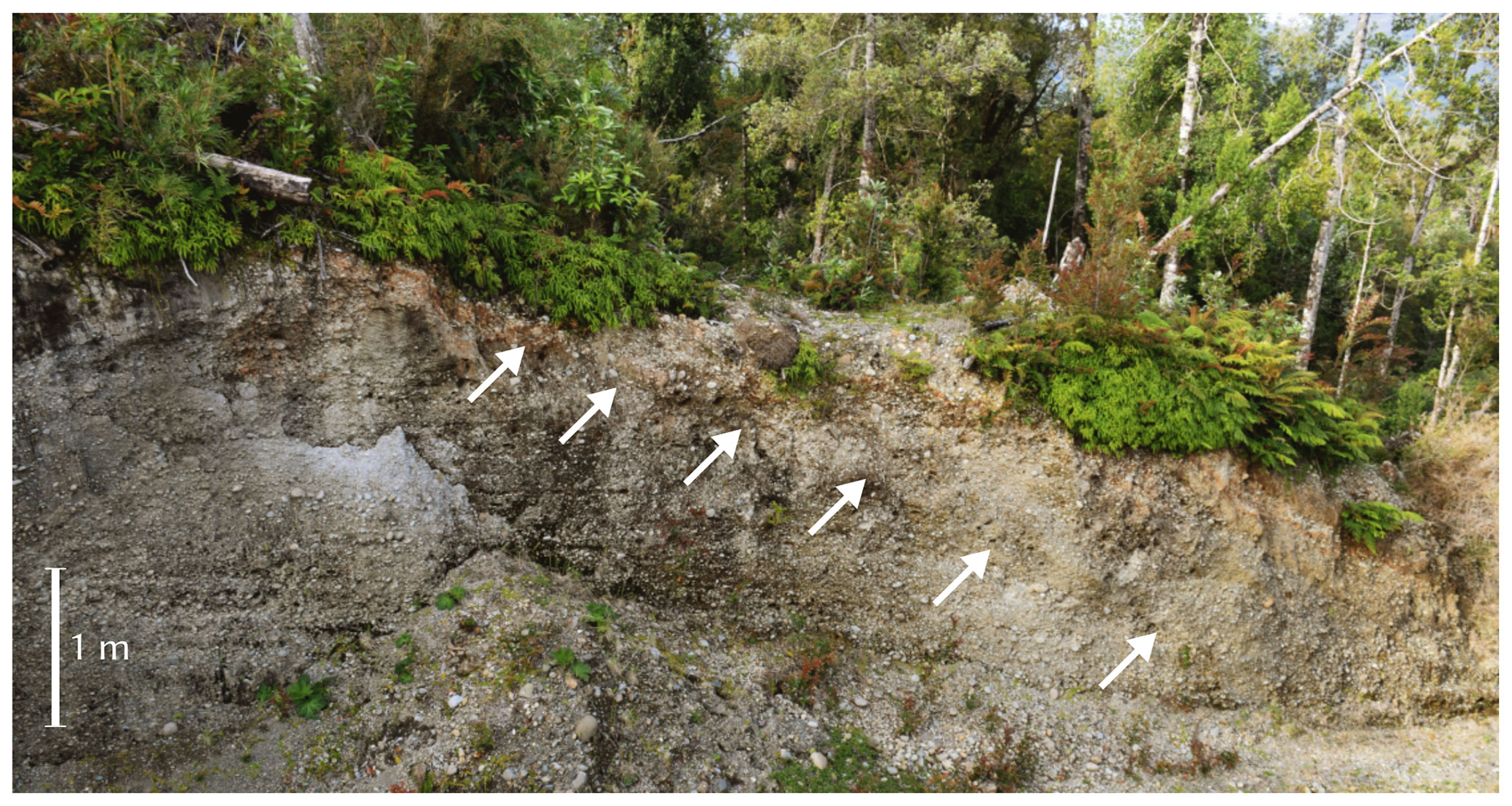
Figure 8 Site Cucao_T1_4 stratigraphic section. The image shows the two main sediment units described here. An outwash of gravel and sand (Gt, St) underlie melt-out till (Dmm); both units are separated by an ice-contact surface (white arrows), suggesting overriding ice.

Interpretation. Gt–St facies in Sect. 4 are related to a channel fill. Being deeper and wider than most channels described so far, these facies could relate to the main route feeding the distributary system alluded to before. The erosion surface towards the terrace edge is interpreted as an ice-contact surface capped by melt-out till (Dmm).

3.1.5 Sites Cucao_T2_5 and _6

Both sites occur within the edge of Cucao_T2 terrace, near the southern coast of Lake Cucao (Fig. 3a). Exposed sediments are very similar, consisting of a series of laterally extensive, 0.1–0.5 m thick sand and pebble beds (Fig. 7g). Beds are mostly composed of a fining-upwards sequence grading from gravel (pebbles and small cobbles) to sand. Sediment is moderately to well sorted, rounded and mostly clast-supported. Channel-shaped bodies 3–5 m wide filled with lateral accretion deposits (St-Sp; Gt-Gp) are fairly common. Beds stack on each other with flat, sharp contacts or low-angle surfaces. There are occasional channel-shaped bodies, 1–2 m thick, filled with well-rounded, well-sorted cobbles.

Interpretation. Dilute stream flow processes within a braided river system. This is the classical sandur deposit within a distal ice-margin environment.

3.1.6 The Till site

This site is located on the southern side of the Chonchi-Queilén route to the east of central Isla de Chiloé (Figs. 1 and 3b). It is a sediment pit 1.5 km to the south after the detour to Las Lajas. The pit was excavated in the southwestern side of a glacially molded hill. A hummocky terrain betters characterized the surroundings including kilometer-scale hills standing several tens of meters above surrounding elongated depressions (Fig. 3b). The excavation walls expose several meters of indurated gravel-rich glacial diamictons making up most of the morainic relief. Sediment structures including a fissility appearance, rudimentary bedding, and well-faceted and striated clasts can be best interpreted as subglacial traction till (Fig. 9) (Menzies, 2012; Menzies et al., 2006; Evans et al., 2006). Intercalated laminated fine sediment occurs within the section, but this is not widespread.

Figure 9 The Till site stratigraphic section. (a) Geomorphic context of the section (red box) on the distal side of a drumlinoid landform (view to the south from the Las Lajas site). Ice flowed from the left (east). (b) Detail of the subglacial till making up most of the sediment section.

3.1.7 Las Lajas site

García (2012) first described this site, located by the Las Lajas detour on the Chonchi-Queilén route (Figs. 3b and 10). It includes two glacial diamictons that sandwich an 80 cm thick peat layer. Whereas the lower diamicton–peat surface contact shows a disconformity, higher up the peat grades conformably into glaciolacustrine sediments and sands overlain by the upper diamicton. The ¹⁴C dates from the base and top of the peat yielded 28.2±0.4 and 25.7±0.4 cal kyr BP, respectively.

Figure 10 Stratigraphic column of the Las Lajas site. Two diamictons (Dmm) sandwich a peat soil (P) and inorganic glacial finer sediments (Sm, Fl). The upper peat layer dates a glacial advance on the site as evidenced by the upward coarsening of the sediments. Modified from García (2012).

3.2 Chronology

3.2.1 Radiocarbon dating

We obtained a total of nine ¹⁴C samples from Cucao_T1 and Cucao_T2 sites (Table 3). In Site Cucao_T1_3 two bulk ¹⁴C samples from a single organic clast embedded in outwash sediment yielded 27.7±0.2 and 31.5±0.3 cal kyr BP, respectively. This clast was embedded in the sediment section nearby where we obtained the luminescence and ¹⁰Be samples (see below). Also in Site Cucao_T1_3, we obtained three ¹⁴C samples from wood pieces protruding out from the upper organic soil unit which ranged from 0.2±0.07 to 7.5±0.07 cal kyr BP. Site Cucao_T1_7 is a rather small (few tens of centimeters thick) sediment exposure on a road side where peat with wood outcrops on top of the Cucao_T1 terrace surface. The ¹⁴C ages of three wood samples ranged from 44.7±0.8 cal kyr BP to >45.0 ¹⁴C kyr BP.

Table 3 The ¹⁴C dates from this study.

In Cucao_T2, we obtained an age of 4.9±0.07 cal kyr BP from the organic soil unit overlying the outwash sediment in Site Cucao_T2_6.

3.2.2 Luminescence dating

We obtained a total of six luminescence samples in both Cucao_T1 (sites Cucao_T1_1–_3) and Cucao_T2 (sites Cucao_T2_5 and _6). The results from high-resolution, low-level gamma spectrometry are summarized in Table 4. All samples were found to be in secular equilibrium. With regard to the equivalent dose determination, all samples showed indicators for incomplete bleaching prior to burial (right skewed dose distributions and high overdispersion values >50 %). Because of that, all equivalent doses were calculated using the bootstrapped MAM (Galbraith et al., 1999; Cunningham and Wallinga, 2012). The age and dose-rate calculation was done using the software ADELE (Kulig, 2005). All ages were corrected for fading using the approach of Huntley and Lamothe (2001). All details are provided in Table 5.

Table 4 Results from radionuclide analysis and dose-rate calculation.

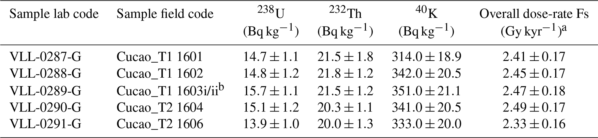
^a Cosmic dose rate determined according to Prescott and Stephan (1982) and Prescott and Hutton (1994), taking the geographical position of the sampling spot (longitude, latitude, and altitude), the depth below surface and the average density of the sediment overburden into account. An uncertainty of 10 % was assigned to the calculated cosmic dose rate. External and internal dose rate calculated using the conversion factors of Adamiec and Aitken (1998) and the β-attenuation factors of Mejdahl (1979), including an α-attenuation factor of 0.08±0.01, an internal K content of 12.5±0.5 % (Huntley and Baril, 1997) and an estimated average water content of 15±5 % throughout burial time. Values covering almost dry to almost saturated conditions. Error was propagated to the overall dose-rate calculation. ^b Only sample Cucao_T1 1603i was measured because both samples were taken in direct vicinity from the same sediment layer.

Table 5 Summary of IR-50 data.

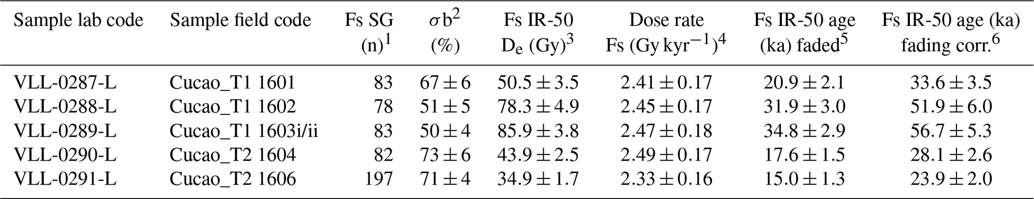
¹ Number of single grains (SGs) passing all rejection criteria. ² Overdispersion calculated using the CAM (Galbraith et al., 1999). ³ Equivalent dose (D_e) calculated using the bootstrapped MAM-3 (Galbraith et al., 1999; Cunningham and Wallinga, 2012) for all samples. ⁴ Overall dose rate. ⁵ Ages calculated using the software ADELE (Kulig, 2005). ⁶ Fs-based ages corrected for fading according to the method of Huntley and Lamothe (2001) using the R luminescence package (Kreutzer et al., 2012)

At Site Cucao_T1_1 we obtained a sample (VLL-0287-L – Cucao-T1-1601) from a sand unit 100 cm below the surface and derived an age of 33.6±3.5 ka. At Site Cucao_T1_2, a single sample (VLL-0288-L – Cucao-T1-1602) was obtained from a sand lens 255 cm below the surface and yielded an age of 51.9±6.0 ka. At Site Cucao_T1_3, we obtained two samples (VLL-0289-L – Cucao-T1-1603 i and ii of which only i was dated) from the same sand unit at 350 cm below surface which yielded an age of 56.7±5.3 ka. From the lower Cucao_T2 terrace, an age of 28.1±2.6 ka was obtained at Site Cucao_T2_5 (VLL-0290-L – Cucao-T2-1604) and of 23.9±2.0 ka at Site Cucao_T2_6 (VLL-0291-L – Cucao-T2-1606) at 1000 and 600 cm below surface, respectively.

3.2.3 The ¹⁰Be depth profile dating

Figure 11a shows that the ¹⁰Be concentration declines exponentially with depth, consistent with post-deposition isotope production in a stable outwash plain and no mixing of sediment. One exception occurred towards the base of the profile where some sediment mixing could have occurred as higher concentration of ¹⁰Be were measured here. Our experiments show that the modeled ¹⁰Be age seems somewhat sensitive to the position of the original outwash surface below the top organic soil unit (20 or 35 cm) and to a lesser degree to the sediment density (1σ range between 1.9 and 2.2 g cm⁻³) (Fig. 11b iv). The modeling yielded low values for ¹⁰Be inheritance (1σ range between 0 and 11 000 ¹⁰Be atoms g⁻¹, as expected in glacial sediments; Fig. 11b iii). Based on these boundary conditions, the Cucao-T1 outwash age ranges between 45 and 100 ka (Fig. 11i, c), conditioned by the age of the organic soil formation. Accordingly, if the soil formed or was present as it is today for a short time (i.e., centennial to millennial timescales), the Cucao-T1 age would be closer to the younger limit (45 ka); alternatively, if the soil formed together with the outwash abandonment, the Cucao-T1 age would be closer to the older limit (100 ka). All other possible scenarios for organic soil formation would yield intermediate ages for Cucao-T1 outwash deposition (between 45 and 100 ka).

Figure 11 Site Cucao_T1_3 ¹⁰Be depth profile results. (a) Depth profile with cosmogenic samples and vertical distribution of the outwash and the overlaying organic sediments: Be-10 data in blue, best fit of the Be-10 accumulation models in green and 1σ fitting models in grey. (b) Probability density distributions of the parameters considered in the models shown in (a). (c) The 1σ results of the fitting ages for the deposition of the outwash and the organic layer in different shades of grey based on their probabilities.

4 Discussion

4.1 The Cucao_T1 and Cucao_T2 ages

Based on the ¹⁴C ages obtained for the peat unit capping the outwash sediment at Site Cucao_T1_7, we can determine that fluvioglacial activity linked to Cucao_T1 ended by 44.7±0.8 to >48.3 cal kyr BP. In other words, the outwash minimum age is the ¹⁴C saturation age. This minimum age based on radiocarbon agrees with the depositional luminescence ages of 51.9±6 and 56.7±5.3 ka (Cucao-T1-1602 and Cucao-T1-1603 i) which occur near the younger ¹⁰Be model age limit. The two luminescence ages are in good agreement within error, which strengthens the reliability of the ages and the chosen luminescence dating approach. The IR-50 age obtained for Cucao-T1-1601 yielding 33.6±3.5 ka is not in agreement with the previous reasoning. Because all methodological steps involved to obtain that age are in agreement with the quality criteria applied for all luminescence samples in this study, the age must be regarded as a reliable luminescence age from a methodological point of view. However, there are a number of environmental uncertainties which may explain the age underestimation of that sample: this sample was taken close to the sediment surface at approximately 1 m depth. Bioturbation (plant roots, digging activities of animals) may be relevant when a sample is taken close to the surface. Although no indication of such processes was detectable in the field, it cannot be ruled out that grains from the soil surface may have been relocated to deeper layers by bioturbation processes. This would result in a shift of the equivalent dose distribution to a lower dose which corresponds to a younger age. A second scenario might be that the sediment of the Cucao-T1-1601 site was locally redeposited in an event not related to the primary terrace formation. As there is no age control from radiocarbon at that site, this may have to be considered as a valid option and is further discussed in the context of the formation of the Cucao_T2 terrace level. Considering the ¹⁴C ages from Site Cucao_T1_7, it is clear that the Cucao-T1-1601 IR-50 sample must be regarded as a minimum age for the Cucao_T1 terrace formation.

In order to determine the age of the Cucao_T1 terrace, we have considered two different scenarios (“a” and “b”) that best reconcile the ¹⁴C, IR-50 and ¹⁰Be chronologies obtained for this outwash. For both scenarios we have calculated the probability distributions in Bayesian terms. In both scenarios, all ages obtained for the Cucao_T1 outwash deposition are older than the ¹⁴C ages from Site Cucao_T1_7. The scenario “a” considers the ¹⁰Be age as a minimum (i.e., corresponding to a short-lived organic soil development) and the luminescence ages as the depositional age of the outwash sediment. The scenario “b” considers the wide ¹⁰Be age range (i.e., corresponding to an organic soil development at any time since the Cucao_T1 outwash abandonment), together with the luminescence ages, as the depositional ages of the outwash. For scenario “a”, the resulting age is 57.8±4.7 ka, and for scenario “b” the resulting age is $\mathrm{55.5}\begin{array}{c}+\mathrm{29}\\ -\mathrm{6.5}\end{array}$ ka.

The data show that both scenarios yield statistically the same most likely age but differ in precision (Figs. 12a, b). The overlap between luminescence ages and ¹⁰Be fitting models (youngest outwash ages in Fig. 11c) suggest that most of the organic soil unit has been in its present form and thickness for a limited time span. The older ¹⁴C ages (Site 7) also suggest that scenario “a” is most probable, which implies that the shielding of cosmogenic radiation by the organic unit has not been significant since the Cucao_T1 outwash deposition (MIS 3). A question may arise regarding the range of ¹⁴C ages we obtained from the organic sediment capping the Cucaco_T1 outwash in two different sites, including MIS 3 (Cucao_T1_Site 7) and Holocene (Site 3) dates. Taking the data at face value, and in the light of ¹⁰Be and IR-50 data, it is unlikely that an organic soil as thick (and dense) as in Site Cucao_T1_7 has been present since $\ge \mathrm{48.3}\pm \mathrm{1.3}$ cal kyr BP. The implication is that the top organic soil was not preserved throughout the MIS 3 and MIS 2 until the present. In fact, we do not find MIS 3 but only Holocene ¹⁴C ages in Site 3, supporting a young organic cover (Table 3). This points to an unsteady organic layer cover (e.g., mostly absent or of limited thickness) after the Cucao_T1 deposition. Therefore, our preferred modeled age, when IR-50, ¹⁰Be and ¹⁴C data match, is 57.8±4.7 ka for the Cucao_T1 outwash deposition. This age identifies the early Llanquihue Glaciation in Chiloé (i.e., the lLGM).

Figure 12 Scenarios “a” and “b” probability distributions of ¹⁰Be, ¹⁴C and IR-50 data. Both scenarios coincide in the best Bayesian age but differ in terms of precision. In (a), scenario “a” considers that the organic soil as it is today has been present in the site for only a short time (centuries to millennia). The kernel density estimation of the age of the outwash has been calculated as $p\left(\text{TOSL}\right|t)\cdot p(T{}^{\mathrm{14}}\mathrm{C}<t)\cdot p(T{}^{\mathrm{10}}\mathrm{Be}<t)$, where p(TOSL|t) is the sum of the probabilities corresponding to the IR-50 ages, and p(t>T¹⁴C) and p(t>T¹⁰Be) are the cumulative sum of the probabilities corresponding to the minimum ¹⁴C and ¹⁰Be ages, respectively. In this case, we only considered the probabilities of the minimum ¹⁰Be age corresponding to an age of 0 for the organic soil (y=0 in Fig. 11c; 56.5±8.5 ¹⁰Be ka). In (b), scenario “b” considers that the organic soil was formed anytime between outwash deposition and today. The kernel density estimation of the age of the outwash has been calculated as $p\left(\text{TOSL}\right|t)\cdot p(T{}^{\mathrm{14}}\mathrm{C}<t)\cdot p(T{}^{\mathrm{10}}\mathrm{Be}\left|t\right)$, where p(T¹⁰Be|t) corresponds to the ¹⁰Be age obtained in Fig. 11 (72.5±26.5 ¹⁰Be ka). Note that here only the ¹⁴C ages are considered as minimum ages.

The two luminescence IR-50 ages obtained from samples related to the Cucao_T2 terrace yielded ages in good agreement within error. The calculated mean age of 26.0±2.9 ka obtained for the Cucao_T2 terrace corroborates that this terrace represents a younger, inboard glacial extent. The increased geomorphic activity in the area during the formation of the Cucao_T2 terrace level likely included enhanced incision into the Cucao_T1 terrace level and increased remobilization of sediments on the Cucao_T1 terrace. This initial phase of climate deterioration potentially resulted in the remobilization of material on the Cucao_T1 terrace level, followed by incision and subsequent build-up of the Cucao_T2 terrace on a lower level. The initial phase of remobilization and incision may be represented by the IR-50 age of sample Cucao-T1-1601, which was taken close to the present Cucao_T1 terrace surface (and present-day Cucao_T1–Cucao_T2 scarp) and yielded an age of 33.6±3.5 ka, which is only slightly older than the luminescence ages obtained from the Cucao_T2 terrace sediments.

4.2 The local LGM ice limit

Based on the mapping, sediment preservation and age of the landforms, each Cucao outwash plain Cucao_T1 and Cucao_T2 could be linked to expanded ice marginal positions within the last glacial period (Fig. 3a). García (2012) mapped a double Llanquihue age ice-contact slope widespread on the eastern slope of the Cordillera de la Costa that was linked to a double system of outwash terraces on the western mountainside, such as Cucao_T1 and Cucao_T2. In this scenario, the PIS buttressed against the Cordillera de la Costa (here up to ∼500 m a.s.l.), which acted as a barrier for the Golfo de Corcovado Ice Lobe's expansion towards the open Pacific Ocean. The mountain range is punctuated by meltwater channels that grade to the outwash plains to the west. Opposite, the Huillinco–Cucao basin (Fig. 1) allowed a narrow tongue of ice to flow through the coastal mountains. Here, the exact ice marginal positions attained during the Cucao_T1 and Cucao_T2 outwash depositions are not obvious. It is possible that part of the scarp separating Cucao_T1 from Cucao_T2 can be regarded as a reworked ice contact slope (Fig. 3a). Several sources of evidence could support this scenario indicating ice proximity: (1) a glacial diamicton outcropping at the proximal edge of T1 in Site Cucao_T1_4, (2) the Cucao_T1 terrace high dipping angle of ∼2 % and (3) the ice proximal facies (e.g., debris flows) intercalated with better sorted outwash outcroppings in the studied sediment sections within Cucao_T1 terrace (Figs. 7 and 8). On the other hand, the lower Cucao_T2 deposition can be linked to an inboard ice margin at the proximal edge of this outwash plain (Fig. 3a). The morainic relief confining the Quilque lake can be interpreted as a hummocky moraine formed as part of a dead-ice topography related to the deglacial phase after the terminal position against the ice contact slope of Cucao_T1 terrace or, alternatively, as a push complex during active ice recession (Evans and Twigg, 2002). Sediment slumps from the T1 ice-contact slope during a paraglacial phase are also a possibility during deglaciation.

The inferred ice limits imply that ice reached more or less similar positions, first at 57.8±4.7 ka (Cucao_T1 terrace) and then 26.0±2.9 ka (Cucao_T2 terrace), with ice covering most of the island to the Cordillera de la Costa or slightly beyond this point along the Huillinco–Cucao basin.

An extended ice position to the Cordillera de la Costa at 26.0±2.9 ka may be in conflict with a previous interpretation of the Las Lajas site (García, 2012). Here, the upper diamicton was interpreted as being deposited at the ice margin by 25.7±0.4 cal kyr BP. This ice advance was preceded by ice-free conditions interpreted from the peat layer between 28.2±0.4 and 25.7±0.4 cal kyr BP when ice should have resided up-glacier from the Las Lajas site (i.e., reduced ice standing to the east of Isla de Chiloé). Then, the Cucao_T2 outwash deposition can only have occurred between 26  cal kyr BP and 23.1 ka, if the age control from both sites (the IR-50 and ¹⁴C ages) is considered using 1σ range. Several lines of evidence suggest that the ice expanded westward to the Cordillera de la Costa by 25.7±0.4 cal kyr BP to deposit the Cucao_T2 terrace. First, it seems difficult to reconcile an ice margin at eastern Chiloé building the western Cucao_T2 outwash plain ≥20 km away. No topographic match seems plausible. Second, ice must have overridden Las Lajas when it expanded westward to the Cordillera de la Costa. Third, nearby sediment and the geomorphic record denote that subglacial morphogenesis originated by overriding ice. The Till site, near Las Lajas, exposes well-preserved subglacial traction till (Figs. 3b and 9). Nearby exposures along the Chonchi-Queilén route in eastern Chiloé (Fig. 1) commonly denote outwash sediments being capped with erosional surfaces by glacial diamictons, showing overriding ice during ice expansion (García, 2012). Fluting and drumlinoid landforms cored by till then can suggest that rapid-flowing ice expanded all the way to the Cordillera de la Costa in central Chiloé during the Llanquihue Glaciation. In the light of the new morphostratigraphic observations and geochronologic data, we thus suggest the Golfo de Corcovado Ice Lobe expanded towards the Cordillera de la Costa to deposit the Cucao_T2 outwash by 25.7±0.4 cal kyr BP, thus overriding central Chiloé during the global LGM. Just north in the CLD, glaciers reached their most extensive positions by about 26 ka also, as suggested by Denton et al. (1999b). Antarctic ice cores show stadial conditions between ∼28 and 24 ka peaking at ∼26 ka that seem to be mirrored by SST offshore Chiloé (WAIS Divide Project Members, 2015; Lamy et al., 2004).

4.3 The pre-LGM Llanquihue Glaciation

Precise geochronologic records of glacial activity during the early to middle MIS 3 are rare in the CLD. Moreover, no records of MIS 4 glaciation exist on land. On the other hand, available radiocarbon data have precisely constrained glacial fluctuations during the LGM (Mercer, 1972, 1976; Porter, 1981; Denton et al., 1999b). Therefore, only a limited understanding of glacial fluctuations during pre-LGM time exists today. Available dating for the early Llanquihue drift is mostly equivocal because either the stratigraphic context is not well understood or dates reported are not sufficiently precise ages for dating putative pre-LGM glacial advance(s) (Porter, 1981; Denton et al., 1999b). For instance, the “crossroad stratigraphic site” west of Lago Llanquihue (Denton et al., 1999b; Porter, 1981; Mercer, 1976) includes deformed weathered pyroclastic organic sediments including wood and charcoal sandwiched by pre-Llanquihue (below) and Llanquihue (above) till. Minimum ages ranging from $>\mathrm{39.6}\pm \mathrm{0.7}$ to 57.8 ¹⁴C kyr BP obtained from the non-glacial sediments do not closely constrain the age of glacial advances represented by the till units. Nearby the “crossroad site”, a reworked organic clast into Llanquihue outwash yielded >44.4 ¹⁴C kyr BP (Denton et al., 1999b; Mercer, 1976). Similarly, the bottom sediments of the Puerto Octay and the Bahía Frutillar Bajo sections show Llanquihue drifts deposited before 41.3±0.7 and 45.4±2.0 cal kyr BP, respectively (Denton et al., 1999b). To the north, an early Llanquihue glacial advance >56.0 ¹⁴C kyr BP occurred in Lago Ranco, as suggested by ¹⁴C dating of a log in peat that occurs stratigraphically linked to interpreted till sediments (Mercer, 1976). Porter (1981) reported a wood age of 45.7±1.0 cal kyr BP from an interdrift in situ stump in Punta Penas. In Punta Pelluco, wood in a similar stratigraphic context yielded >40.0 ¹⁴C kyr BP (Porter, 1981). All these records suggest Llanquihue glacial expansions during pre-LGM times, but it remains unclear the precise dates of the events. In contrast, the Taiquemó record in Chiloé provides unique details regarding the Llanquihue Glaciation (Heusser et al., 1999). The Taiquemó mire is located inboard from the outermost early Llanquihue moraine. The basal minimum limiting age of Taiquemó of >49.9 ¹⁴C kyr BP suggests this early Llanquihue landform was deposited by this time. Dating of the Taiquemó basal sediments beyond the ¹⁴C technique suggest that an early glacial maximum occurred before >50.0 ¹⁴C kyr BP when a pollen peak in Gramineae overlaps with a jump in magnetic susceptibility and a minimum in loss on ignition (Heusser et al., 1999).

Although dating control is limited (i.e., available dates occur at the limit and beyond the ¹⁴C possibilities, >50 ¹⁴C kyr BP), evidence suggests that interstadial periods dominated by tree species adapted to cool and humid conditions occurred during the MIS 3 (Heusser et al., 1999; Villagrán et al., 2004, 2019). A reasonable scenario is that these ecosystems spread during the Antarctic millennial-scale interstadial periods that punctuated the MIS 3, for instance, at ∼60 ka (Antarctic Isotope Maximum, AIM, 17) and/or at ∼54 ka (AIM 14) (WAIS Divide Project Members, 2015). Near the base of the Taiquemó record a peak in warm temperatures was interpreted from a broad peak in loss of ignition and a Gramineae minimum within subantarctic evergreen forest conditions (Heusser et al., 1999) which could have been accompanied by the expansion of conifer forest to the low lands of Chiloé (Villagrán et al., 2004). Therefore, we suggest that the Cucao_T1 glacial advance was triggered by a millennial-scale climate deterioration that followed an interstadial peak (e.g., the AIM 17). This PIS glacial expansion by 57.8±4.7 ka into the outermost ice-contact slope in Chiloé coincided with a decreasing SST trend that lasted several millennia and culminated offshore Chiloé ∼ 4–5 ^∘C below the early Holocene value (Kaiser et al., 2005). The Antarctic temperature stack (Parrenin et al., 2013), which mimics the WAIS divide ice core δ¹⁸O record (WAIS Divide Project Members, 2015), records a stadial period culminating at ∼57 ka when atmospheric temperatures reached 6–7^∘C below those of the present day. Presumably, during this Antarctic stadial the westerly wind belt shifted north, associated with extended sea ice and the expansion of Antarctic and subantarctic atmospheric and oceanic conditions into lower latitudes (Lamy et al., 2015). The expanded westerly wind belt linked to an enhanced northern ACC boundary brought depressed SST and air temperatures and high precipitation to the latitude of Chiloé, thus forcing a PIS advance here by the early MIS 3.

4.4 MIS 3 paleoclimate

This section discusses the MIS 3 paleoclimate in the context of glacial fluctuations of the PIS and other Southern Hemisphere mountain glaciers. Globally, the MIS 3 is a long-term interstadial phase when ice sheets were reduced, sea level reached intermediate stands, and temperatures were mild (Shackleton et al., 2000; Ivy-Ochs et al., 2008; Parducci et al., 2012; Dalton et al., 2019). The peak of the MIS 3 warmth occurred at ∼60 ka, the first in a sequence of prominent millennial-scale climate changes (e.g., Dansgaard–Oeschger and AIM events) recorded at both polar hemispheres during this period (Jouzel et al., 2007). Nonetheless, the climate variability in the MIS 3 is conspicuous not only in the polar records but elsewhere (Mayr et al., 2019).

After MIS 4, climate in New Zealand and southern Chile was rather mild. In New Zealand, the Aurora Interstadial lasted until about 43 ka, but it was interrupted by stadial conditions, first at 49–47 ka and then at 42–38 ka, when Southern Alps glaciers readvanced (Williams et al., 2015; Kelley et al., 2014; Doughty et al., 2015). Between 37–31 ka, a new phase of mild interstadial temperatures was recorded in New Zealand, after which temperatures declined into the MIS 2 global LGM phase (Putnam et al., 2013; William et al., 2015; Darvill et al., 2016). In southern Chile, Heusser et al. (1999) recorded interstadial temperatures and humid conditions until about >50 ka when temperatures started a cooling trend that extended until the global LGM. Ice-free areas later overridden by glacier or ice proximal outwash deposits occurred between about 43–33 ka, thus indicating mid-to-late MIS 3 ice fluctuations (Denton et al., 1999b). Similarly, high and low frequencies of Gramineae punctuated the MIS 3, thus being indicative of millennial-scale temperature changes throughout the MIS 3 (Heusser et al., 1999). Distal to the PIS front, interstadial conifer forests are known to have grown in areas later overridden by ice, as recorded by peat layers containing tree trunks on sea-cliff exposures and also by tree stumps standing in life position at present-day intertidal sea shores (Roig et al., 2001; Villagrán et al., 2004, 2019). Along the eastern coastal cliffs of Chiloé multiple peat layers are intercalated with finely laminated glacial sediments assumed to be early MIS 3 in age, suggesting short-term environmental variability (Villagrán et al., 2004, 2019). Moreover, these glacial-sourced sediments suggest that the PIS front, although located up ice from Isla de Chiloé, was not much further to the east during the MIS 3. A similar conclusion can be derived from the alternating peat and lake facies that punctuate the Taiquemó record between about > 50–40 ka (Heusser et al., 1999). Altogether, the available records show that not only did mild atmospheric conditions punctuate the MIS 3, but rather this was a variable climatic period both in the middle and high latitudes. In fact, Lovejoy and Lambert (2019) noted that the highest climate variability occurs during the middle of a glacial cycle (e.g., MIS 3), the opposite being true at the ends (i.e., the LGM) when a rather stable climate predominates. These authors studied the European Project for Ice Coring in Antarctica (EPICA) dust flux frequency record, which is known to be linked to Patagonian climate and glacial fluctuations, among others factors (Lambert et al., 2008), and which therefore provides a direct link between southern middle and high latitudes (Sugden et al., 2009; Kaiser and Lamy, 2010). During mid-glacial climates, transition times and amplitudes of Antarctic dust flux variability occurred at centennial to millennial timescales implying that large PIS ice lobe extent variability occurred also at these time frequencies in response to climate change forcing (see Lovejoy and Lambert, 2019). Therefore, an extensive northern PIS glacial expansion at 57.8±4.7 ka in Chiloé, together with that recorded by the PIS in Torres del Paine, Última Esperanza and Bahía Inútil by ∼48 ka (Sagredo et al., 2011; Darvill et al., 2015; García et al., 2018) and in New Zealand at ∼ 49–47 and 42–38 ka (Kelley et al., 2014; William et al., 2015), suggests a distinct return to glacial conditions in the southern midlatitudes within the MIS 3.

5 Conclusions

Full glacial advances by the Golfo de Corcovado Ice Lobe of the northwest Patagonian Ice Sheet (PIS) occurred by 57.8±4.7 and 26.0±2.9 ka on the Isla de Chiloé and respectively deposited the outer Cucao_T1 and Cucao_T2 outwash plains enclosing the Lago Cucao basin. The latter ice advance could be tied to a previously dated advance to 25.7±0.3 cal kyr BP that better constrains its age (García, 2012). The extent of the now inexistent Golfo de Corcovado Ice Lobe was >100 km during both glacial expansions, which did not reach the Pacific Ocean during the Llanquihue Glaciation. The early Llanquihue ice expansion during the MIS 3 occurred intercalated with interstadial periods, which denotes the sensitive response of the Patagonian glaciers to centennial- to millennial-scale climate fluctuations. Southern midlatitude glacial advances interrupting the apparent mild climate that characterized the early MIS 3 imply that this time period was rather characterized by large and rapid climate oscillations not only at the poles but elsewhere.