the Creative Commons Attribution 4.0 License.
the Creative Commons Attribution 4.0 License.
 | 26 Jan 2024
MiGIS: micromorphological soil and sediment thin section analysis using an open-source GIS and machine learning approach
Marie Gröbner
Astrid Röpke
Martin Kehl
Zickel, M., Gröbner, M., Röpke, A., and Kehl, M.: MiGIS: micromorphological soil and sediment thin section analysis using an open-source GIS and machine learning approach, E&G Quaternary Sci. J., 73, 69–93, https://doi.org/10.5194/egqsj-73-69-2024, 2024.
Micromorphological analysis using a petrographic microscope is one of the conventional methods to characterise microfacies in rocks (sediments) and soils. This analysis of the composition and structure observed in thin sections (TSs) yields seminal, but primarily qualitative, insights into their formation. In this context, the following question arises: how can micromorphological features be measured, classified, and particularly quantified to enable comparisons beyond the micro scale? With the Micromorphological Geographic Information System (MiGIS), we have developed a Python-based toolbox for the open-source software QGIS 3, which offers a straightforward solution to digitally analyse micromorphological features in TSs. By using a flatbed scanner and (polarisation) film, high-resolution red–green–blue (RGB) images can be captured in transmitted light (TL), cross-polarised light (XPL), and reflected light (RL) mode. Merging these images in a multi-RGB raster, feature-specific image information (e.g. light refraction properties of minerals) can be combined in one data set. This provides the basis for image classification with MiGIS. The MiGIS classification module uses the random forest algorithm and facilitates a semi-supervised (based on training areas) classification of the feature-specific colour values (multi-RGB signatures). The resulting classification map shows the spatial distribution of thin section features and enables the quantification of groundmass, pore space, minerals, or pedofeatures, such nodules being dominated by iron oxide and clay coatings. We demonstrate the advantages and limitations of the method using TSs from a loess–palaeosol sequence in Rheindahlen (Germany), which was previously studied using conventional micromorphological techniques. Given the high colour variance within the feature classes, MiGIS appears well-suited for these samples, enabling the generation of accurate TS feature maps. Nevertheless, the classification accuracy can vary due to the TS quality and the academic training level, in micromorphology and in terms of the classification process, when creating the training data. However, MiGIS offers the advantage of quantifying micromorphological features and analysing their spatial distribution for entire TSs. This facilitates reproducibility, visualisation of spatial relationships, and statistical comparisons of composition among distinct samples (e.g. related sediment layers).
Die mikromorphologische Analyse mithilfe eines petrografischen Mikroskops gehört zu den konventionellen Methoden um Mikrofazies in Gesteinen (Sedimenten) und Böden zu charakterisieren. Die Analyse des Inhalts und der Struktur anhand von Dünnschliffen (TSs) liefert wegweisende, jedoch größtenteils qualitative Daten zu deren Bildung. In diesem Zusammenhang stellt sich die Frage: Wie können mikromorphologische Merkmale gemessen, klassifiziert und vor allem quantifiziert werden, um Vergleiche über die Mikroskala hinaus zu ermöglichen? Mit dem Micromorphological Geographic Information System (MiGIS) haben wir eine auf Python basierende Toolbox für die Open-Source-Software QGIS entwickelt, die eine unkomplizierte Lösung bietet, um mikromorphologische Merkmale (Features) in TSs digital zu analysieren. Durch die Verwendung eines Flachbettscanners und (Polarisations-) Folie lassen sich hochauflösende RGB-Bilder im Durchlicht (TL), polarisierten Licht (XPL) und reflektiertem Licht (RL) Modus aufgenehmen und verarbeiten. Durch die Zusammenfassung dieser Aufnahmen in einem Multi-RGB Raster können dann Feature-spezifische Bildinformationen (z.B. Lichtbrechungseigenschaften von Mineralen) in einem Datensatz kombiniert werden. Dieser bietet die Grundlage für die Bildklassifikation mit MiGIS. Das MiGS-Klassifikationsmodul nutzt den Random Forest Algorithmus und ermöglicht eine halbüberwachte (auf Trainingsflächen basierende) Klassifizierung der Feature-spezifischen Farbwerte (Multi-RGB-Signaturen). Daraus resultiert eine Klassifikationskarte, welche die räumliche Verteilung der Features im Dünnschliff zeigt und eine Quantifizierung von Grundmasse, Porenraum, Mineralen oder pedogenen Merkmalen (Pedofeatures) wie Eisenoxidkonkretionen und Tonkutanen ermöglicht. Wir demonstrieren die Vorteile und Grenzen der Methode anhand von TSs aus einer Löss-Paläosol-Sequenz in Rheindahlen (Deutschland), die zuvor mit konventionellen mikromorphologischen Techniken untersucht wurde. Hier zeigt sich, unter Beachtung der hohen Farbvarianz innerhalb der Feature-Klassen, dass MiGIS für diese Sedimente gut geeignet ist und somit genaue TS-Feature Karten erstellt werden können. Die Klassifikationsgenauigkeit kann allerdings durch die TS-Qualität und den mikromorphologischen Kenntnisstand bei der Erstellung der Trainingsdaten variieren. Im Allgemeinen bietet MiGIS jedoch den Vorteil, dass mikromorphologische Merkmale quantifiziert und deren räumliche Verteilung für den gesamten TS analysiert werden können. Dies ermöglicht eine Reproduzierbarkeit, Visualisierung räumlicher Beziehungen und statistische Vergleiche der Zusammensetzung zwischen verschiedenen Proben (z.B. aus ähnlichen Schichten).
- Article
(8948 KB) - Full-text XML
- Companion paper
- BibTeX
- EndNote


A common task in petrography, sedimentology, and soil science is the microscopic characterisation of rocks (sediments) or soils aiming to describe the overall composition, facies type, or pedogenic features of the materials. This can provide valuable clues on their nature and formation. The analysis is usually done under the optical microscope using polarisation techniques (i.e. a petrographic microscope) and thin sections (TSs) prepared from the sample. While the principal optical techniques originate in petrography, the analytical method has been further elaborated and widely used in soil science and palaeopedology, where it is known as soil micromorphology (e.g. Bullock and International Society of Soil Science, 1985; FitzPatrick, 2012; Stoops et al., 2018), and more recently in sedimentology (van der Meer and Menzies, 2011) and archaeology (Canti and Huisman, 2015; Courty et al., 1989; Nicosia and Stoops, 2017).
Principally, conventional micromorphological analysis yields qualitative data on the size, shape, arrangement, and count of pores, minerals, and organic matter in the sediment or soil groundmass. This also applies to the analysis of pedofeatures, secondary accumulations that are diagnostic for soil formation (Stoops, 2020). Various light path modes, e.g. PPL (plane polarised light), XPL (cross-polarised light), and OIL (oblique incident light), applied with a petrographic microscope are indispensable to identify and distinguish particles in TSs by their specific light refraction properties (e.g. FitzPatrick, 2012; Ligouis, 2017; Nesse, 2013). This procedure implies that fragmented, microscopic field-of-view observations must be recombined after completion of the TS analysis. In this concern, it is essential to follow accurate documentation and classification guidelines, such as the standards established by Georges Stoops (2020) for micromorphology. As a result, constituent (feature) quantities and spatial relationships, which are important to detect patterns (microstructure, groundmass composition, inclusions, pedofeature abundance, etc.), can be determined. This conventional procedure allows very precise statements on sediment or soil composition with regard to depositional and post-sedimentary formation processes (e.g. Bullock and International Society of Soil Science, 1985; FitzPatrick, 2012; Stoops et al., 2018). However, the conventional approach is laborious and requires intensive academic training. The same applies to the point counting technique, which is a common option to quantify micro-observations or to study spatial relationships (Drees and Ransom, 1994; Pires de Lima et al., 2020; Tang et al., 2020).
Recently, semi-quantitative approaches using standardised forms (e.g. estimation tables) have been employed to quantify micromorphological constituents, thereby enabling the comparison of microfacies (Brönnimann et al., 2020; Lo Russo et al., 2022). Nevertheless, expert analysis can be subjective, and the standardisation of micromorphological descriptions is still low (Stoops, 2020). Quantification and spatial analysis are time-consuming, and interpretations are difficult to reproduce, display, and discuss. Usually, transparency requires a shared microscope session or workshops to study the respective TSs (Shahack-Gross, 2015).
To deal with these challenges, various approaches have already been developed involving the digitisation of TSs, for example by using transmitted light (TL), cross-polarised light (XPL), and reflected light (RL) flatbed scanning (Arpin et al., 2002; Haaland et al., 2018) or microphotography mosaicking techniques (Sauzet et al., 2017). Also, attempts have already been made to establish a microscopic information system (MIS). Tarquini and Favalli (2010) developed such a GIS (geographic information system)-based approach for petrographic analysis. Concerning image classification algorithms, in addition to image segmentation methods (Tarquini and Favalli, 2010; Visalli et al., 2021), significant progress has been made in the field of machine learning (ML) and deep learning, especially for petrographic studies. The successful determination of porosity and mineral composition in rock TSs via the classification of microphotographs using, for instance, DA (discriminant analysis), ANNs (artificial neural networks), CNNs (convolutional neural networks), support vector machine, and random forest algorithms has already been demonstrated (Ghiasi-Freez et al., 2012; Naseri and Rezaei Nasab, 2021; Rubo et al., 2019; Tang et al., 2020). So far only microphotographs, small areas of sedimentological TSs, have been promisingly classified using these approaches (Arnay et al., 2021), whereas, to our knowledge, no advances have been made when it comes to the semi-supervised classification of entire TSs using a combination of TL, XPL, and RL red–green–blue (RGB) imagery. By assessing TL, XPL, and RL information, micromorphological constituents or features can be reliably determined (Stoops et al., 2018). Referring to multispectral imagery in remote sensing, gained extended spectral dimensions are beneficial concerning the application of ML-based image classification (Lillesand et al., 2015). However, this requires the processing of large (high-resolution) data sets. GIS, such as the open-source software QGIS 3, is designed to process extensive data. It provides highly efficient image manipulation, classification algorithms, and the opportunity to analyse spatial patterns. Especially at the macroscopic level spatial relationships between features that are important for interpretations are revealed in the TS.
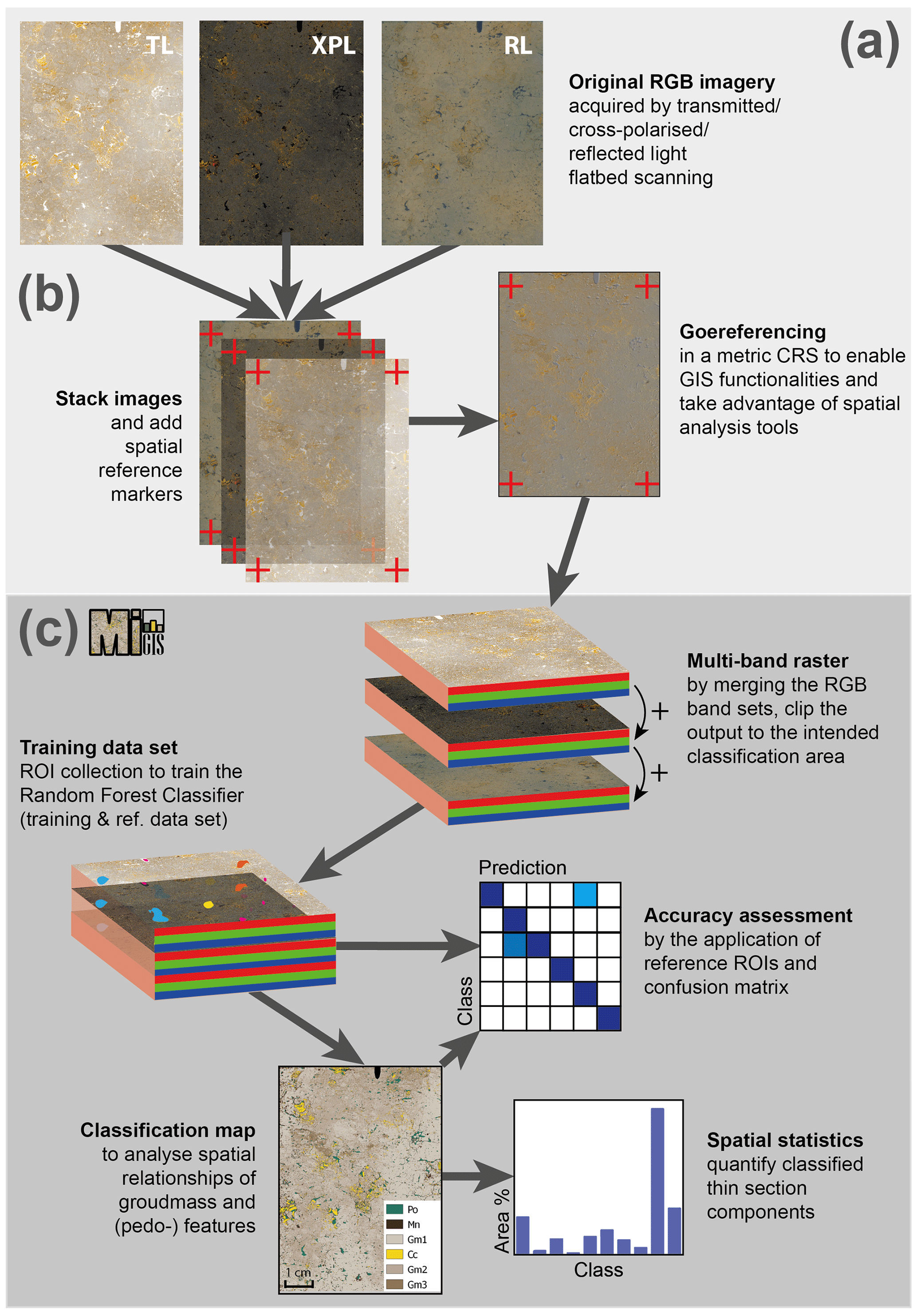
Figure 1Workflow diagram showing digital thin section (TS) analysis principles and main processing steps. TL: transmitted light; XPL: cross-polarised light; RL: reflected light; CRS: coordinate reference system; ROI: region of interest.
Therefore, we developed the Micromorphological Geographic Information System (MiGIS) toolbox, a geoalgorithm processing chain integrable in QGIS 3 (QGIS Development Team, 2022a), which is tailored to handle TS imagery. Our goal was a straightforward and reproducible workflow (Fig. 1) which facilitates GIS integration (Fig. 1b), pre-processing, and training for a random forest algorithm-based semi-supervised classification, as well as accuracy assessment and spatial class statistics (Fig. 1c).
As an auxiliary tool for the conventional approach described above, it should enable the visualisation, quantification, and analysis of spatial relationships of TS constituents. The MiGIS toolbox consists of four Python processing scripts, which can be easily imported to the QGIS processing toolbox.
As a case study, we selected a well-described loess–palaeosol sequence from Rheindahlen in Germany (Kehl et al., 2024). The aim was to classify and quantify the pore space and main micromorphological constituents: four different groundmass types (Gm); coarse constituents, such as medium sand and fine gravel grains (Sg); clay granules (Cg); charred organic material (Ch); and pedofeatures including different clay coating types (Cc, Cci, Ccd) and iron hydroxide (Fe)- and manganese oxide (Mn)-dominated constituents. The methodological advantages of MiGIS are demonstrated using a selection of TSs from Bt horizons.
We composed a digital data set of 21 flatbed-scanned TSs from a 6.5 m thick loess–palaeosol sequence sampled at a former brickyard at Rheindahlen (Germany). The TSs were prepared and analysed in stratigraphic order allowing observations on changes in the type and intensities of soil formation with time. These have already been micromorphologically analysed in detail and described using conventional methods in Kehl et al. (2024). The Rheindahlen sediment sequence contains three different palaeosols characterised by pedogenic illuviation of clay (Bt horizons), which were interpreted to have formed during warmer phases (i.e. interglacials) of the Middle and Late Quaternary. These palaeosols are intercalated in diverse loess deposits that are associated with colder and drier phases (glacials) in the past (Kehl et al., 2024). Undisturbed Bt horizons typically contain coatings of oriented clay minerals (clay coatings), whose specifications and distribution are basically of micromorphological interest because they are evidence of the pedogenic process of clay illuviation (Stoops, 2020; IUSS Working Group (WRB), 2022). From a micromorphological perspective, the samples contain a modest variation of particles, microstructures, and pedofeatures, thus providing a suitable input for our classification test series. The Rheindahlen loess loam exhibits a distinct groundmass mineral composition, featuring a preponderance of angular, spherical grains of silt-sized quartz and feldspar, in addition to elongated mica particles. All TS data sets were classified with MiGIS and statistically evaluated. To illustrate the advantages of a digital TS analysis in detail, a subset of three thin sections of the above-mentioned Bt horizons was selected. TS A4 originates from the modern Bt horizon sampled at a depth of 113 cm below surface (b.s.), B7 was taken from a second Bt (Erkelenz soil) at a depth of 305 cm b.s., and C5 belongs to the third Bt (Rheindahlen soil) extracted from a depth of 524 cm b.s. (Kehl et al., 2024). Since in some cases individual methods, feature classifications, or phenomena are more illustrative in other classified TSs from Rheindahlen, some of these additional results (Appendix B) appear in the figures.
2.1 Micromorphological samples, analysis, and class definitions
High-quality uncovered TSs, 60 mm × 80 mm large and 25 µm thick, were produced by Thomas Beckmann (Schwülper-Lagesbüttel, Germany) involving the impregnation of air-dried sediment blocks with polyester resin under vacuum, hardening over several weeks, as well as cutting, grinding, and polishing as described in Beckmann (1997). Conventional micromorphological analysis (as well as the determination and verification of training areas for the semi-supervised image classification) was accomplished using a polarisation microscope at magnifications of 12.5 ×, 25 ×, 100 ×, 200 ×, or 500 ×, as well as different illumination techniques (PPL, XPL, and OIL). The micromorphological description was carried out according to the protocol and terminology of Stoops (2020). To differentiate between the various clay coating types, appropriate terms suggested by Brewer (1964) were used (Table 1). Features considered in the semi-supervised TS image classification using the MiGIS toolbox in this study are listed and described in Table 1. The feature classes were established based on material screening and conventional micromorphological analysis under the microscope. Corresponding results and interpretations are described in detail in Kehl et al. (2024).
Table 1Micromorphological features observed in thin sections (TSs) from the Rheindahlen loess–palaeosol sequence and class codes for semi-supervised TS image classification.
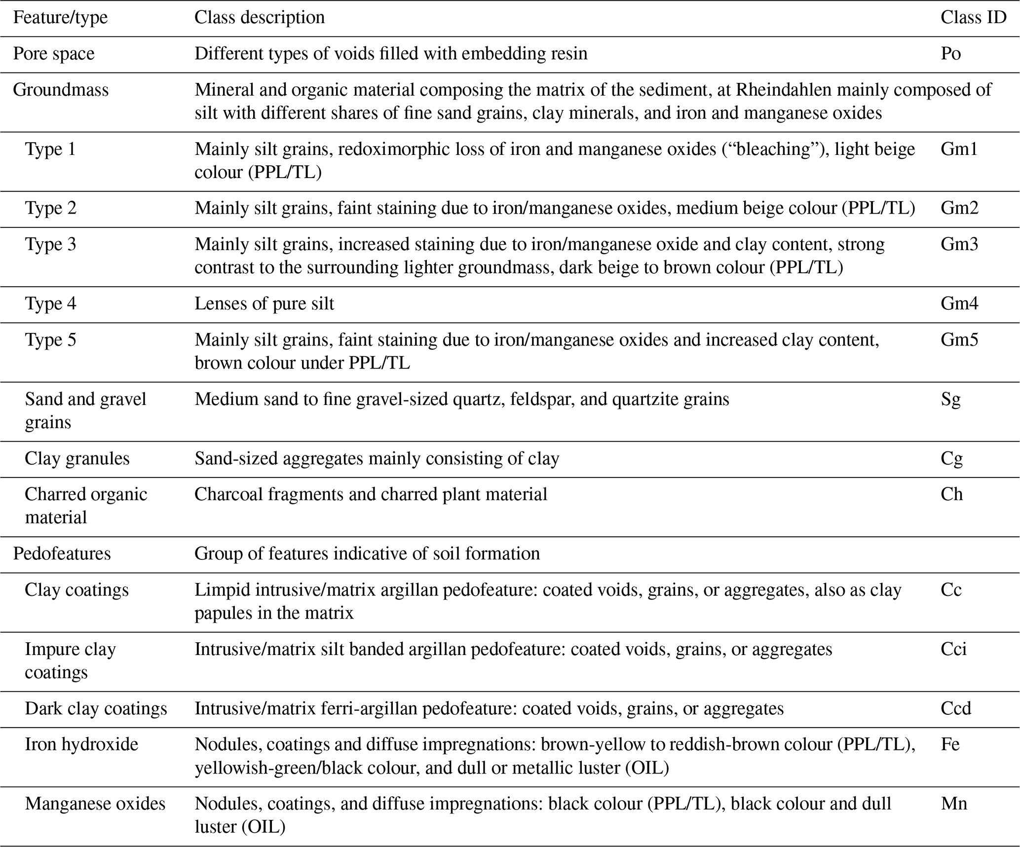
Pore space as observed in TSs under the microscope is less than the total porosity within a sediment or soil horizon due to geometry-related effects such as the Holmes effect or wedging effects (Stoops, 2020). Usually, fine- to medium-sized pore space cannot be detected under the microscope. Indeed, it is assumed that the image classification approach captures a random selection of larger pore cross sections which results in a minimum pore space proportion.
Regarding the groundmass, the resolution limit (here 25 µm) resulting from the section thickness must be taken into account. Since the fine fraction of the groundmass cannot be differentiated due to the overlapping of the particles (Stoops, 2020), we have specified different groundmass types and accordingly created “mixed” training areas for each class (Table 1).
Besides intact clay coatings (Cc), corresponding fragments (clay papules) occur in the sequence and were included in the same class. In addition the class “Fe” represents iron hydroxide.
In general, the colour values of Fe and manganese (Mn) pedofeatures can vary greatly (Vepraskas et al., 2018). In our study, the iron hydroxides appear mainly reddish-brown, whereas manganese-oxide-dominated features appear black under PPL/TL (Stoops, 2020, p. 24). Therefore, we decided to define two separate classes of Fe and Mn pedofeatures depending on their colour under different illumination settings (Table 1).
For each of the listed classes training data were collected (Sect. 2.4.2). If a certain feature class listed in Table 1 was not present in the TS, it was marked with “n/a” (not applicable) in the tabular classification results (Appendix B).
2.2 Thin section imagery acquisition and pre-processing
All TSs were TL scanned (Fig. 1a) with the transmitted light unit of Canon's CanoScan 9000F flatbed scanner, which is a relatively cost-efficient approach compared to professional film scanner and microscopy equipment (Haaland et al., 2018). Apart from test scans using 2400 dpi (Sect. 3.1), the digital scanning resolution was set to 1200 dpi, which represents the maximum optical resolution of the Canon scanner. The resulting RGB image has an approximate pixel ratio of 2801 × 4194 and a pixel size of 0.02 mm × 0.02 mm.
The captured images of 56.02 mm × 83.88 mm and 24 bit colour depth yield in an uncompressed JPG file size of approximately 8 MB. The identical scan resolution should be applied to each TS (TL, XPL, and RL) image of the data set. To produce XPL imagery, two orthogonally oriented polarisation films were positioned below and on top of the TS (Arpin et al., 2002). To obtain surface reflection information (RL), a black plastic sheet was added on top of the section and scanned with the regular flatbed unit. A metal frame (e.g. film holder for transmitted light scans) was applied to keep the TS in an exact position and orientation. If necessary and after capturing the image, contrast and brightness can be adjusted using image processing software. For GIS integration, the TL, XPL, and RL images of each TS must be stacked and supplied with spatial reference points (i.e. crosses; Fig. 1b). To achieve this, we used the open-source image processing software Inkscape. If the resolution and dimensions of each scan are equal, the individual images can be assigned to layers in Inkscape and accurately positioned on top of each other. However, no exact co-registration of the images on pixel scale is required. An additional layer contains the reference points, which needs to be activated before exporting each aligned image. Since the image properties do not have to be adjusted anymore and with regard to a reduced file size, it is recommended to save the images with 8 bit colour depth before processing them in GIS. Concerning the georeferencing process in QGIS, a metric CRS (coordinate reference system) needs to be applied to the previously aligned images. For instance, EPSG:32634 (WGS 84/UTM zone 34N) was used in this study. This is mandatory to obtain realistic metric dimensions for subsequent spatial analysis in GIS. The spatial resolution of 0.02 mm × 0.02 mm (pixel) of the imported images results in clearly visible single features of a size down to approximately 0.1 mm. Below this size, the TS constituents have fuzzy boundaries, but for instance fine sand grains can still be distinguished due to their high interference colours.
Related templates for an Inkscape project and a QGIS Georeferencer POINT data set are provided in the MiGIS repository on GitHub (“Code and data availability” section). These can be used for straightforward georeferencing of 60 mm × 80 mm TS scans with 1200 dpi resolution. Also, detailed instructions on how to stack images and spatial referencing are accessible there.
2.3 Semi-supervised classification of thin section imagery
ML algorithm-based semi-supervised image classification is often used to process remote sensing data, e.g. to create land surface models and other remote sensing products. Using enhanced multispectral information increases the identification accuracy of different surface types, for instance bare soil versus grassland (Lillesand et al., 2015). The expanded spectral data dimension which provides feature-specific spectral signatures enables the classifier to assign pixels with specific values to discrete classes. MiGIS follows a similar approach by using bundled RGB (red–green–blue) information (colour depth) from the TL, XPL, and RL RGB bands, which are composed in a multi-band raster. This raster image thus contains 3 times as much information per pixel as a single image. With only three values (simple RGB image) of, for example, a single TL image, it is likely that the values of different features are too similar in the majority of the channels for a successful division into classes. The extended information in the multi-band raster, on the other hand, allows a clear assignment of a multi-RGB signature for the different features. In Fig. 2 this principle is illustrated by randomly selected single-pixel values for different feature classes.
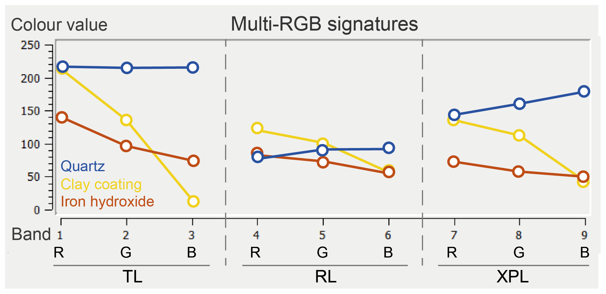
Figure 2Random single-pixel values for different abundant materials in sediment thin sections (TSs) captured from TS A4. The “signatures” of the features are illustrated by artificial lines between the measured pixel values to highlight differences.
To assign pixels to predefined classes (e.g. pore space, clay coating, or manganese) the random forest algorithm needs to be trained by providing a set of regions of interest (ROIs) which cover representative features (pixels) for each class. Based on this data set and using a certain classification scheme, in this case a random forest, the algorithm is able to assign each pixel of the multi-band raster to one of the specified classes.
The implementation of the “Dzetsaka Qgis classification plugin” by Karasiak (2016) in MiGIS enables the use of the random forest classifier of the scikit-learn 1.0.1 Python package (Pedregosa et al., 2011; Scikit-learn developers, 2007–2023) in QGIS 3. The application of feature importance properties and averaging multiple predictions makes the random forest a robust learning method. By default, a fixed number of 100 trees is set, which proved to be a reasonable size to prevent overfitting (Breimann, 2001; Rubo et al., 2019). During the construction each tree is split at every internal node using the square root of the number of features (n):
The features are determined and randomly selected from the training data (n_features): the pixel values defined by the ROIs (regions of interest). The training data set should therefore have a reasonable size. The size depends on the individual data set properties and the desired class number, and there is no standard for this. Nevertheless, it should be taken into account that oversizing can also have negative effects because it will prevent the random forest from learning. The number of samples doubles in each tree level, which results in increased computing time and a fuzzy classification result (Breimann, 2001; Pedregosa et al., 2011; Scikit-learn developers, 2007–2023).
2.4 MiGIS toolbox
Within the toolbox several automated processing steps are covered, ranging from the creation of a cropped multi-band raster, random forest-based image classification, and calculation of class statistics to the accuracy assessment. Originally, MiGIS was composed using QGIS Graphical Modeler (QGIS Development Team, 2022b). Adaptions and extensions of the processing chain have been carried out in Python. The workflow diagram in Fig. 1 illustrates processing steps and the basic principles to apply the presented method. Detailed guidance is available in the MiGIS repository on GitHub (“Code and data availability” section). The four available MiGIS scripts concatenate QGIS 3 (QGIS Development Team, 2022a) and GDAL (GDAL & OGR contributors, 2022) geoalgorithms (both available through the official QGIS 3 repository) in combination with image classification algorithms compiled by Karasiak (2016) within the Dzetsaka Qgis classification plugin. To take advantage of the random forest algorithm in MiGIS the scikit-learn Python package needs to be installed via the QGIS OSGeo4W shell (Windows systems) beforehand (“Code and data availability” section). Detailed references of the applied algorithms are provided in Appendix A.
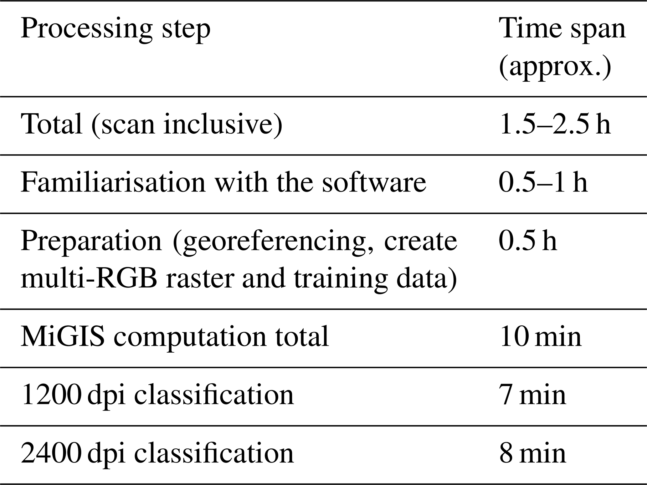
In terms of processing time, the total effort of 1.5 to 2.5 h per TS (Table 2) can be considerably reduced after becoming familiar with the software and the various preparation steps. It should be emphasised that digital processing does not replace detailed micromorphological analysis under any circumstance. Instead, it serves as a tool to enhance classical micromorphological analysis with quantitative, statistically viable data. Simultaneously, it offers a convenient method for feature mapping, a capability not found in semi-quantitative approaches such as point-counting (Drees and Ransom, 1994; Murphy et al., 1977) or comparison with estimation charts. Therefore, it significantly improves the presentation and archiving of collected data in a sustainable and illustrative manner.
Table 2MiGIS processing steps and related time expenditure per sample (Intel i7 processor, 32 GB RAM).
2.4.1 Pre-processing georeferenced thin section images
A cropped multi-band raster, containing the target classification area of the TS (sample section) and multi-RGB information of the TL, XPL, and RL bands, is the centrepiece for a successful classification of micromorphological features in TSs. The tool “MiGIS 1 preprocess TS images” (“Code and data availability” section) facilitates the creation of a multi-band raster with six bands (TL and XPL RGB image) or nine bands (TL, XPL, and RL RGB image). The resulting raster data set can be further refined by clipping it to the extent of a custom vector polygon layer (see Appendix A). Usually, this is the part of the glass slide covered by the sample. Gaps, such as processing artefacts (e.g. drying cracks, label section), should be omitted from the polygon area (QGIS Development Team, 2022b). In this way, irrelevant image parts can be excluded to obtain precise spatial statistics.
2.4.2 The classification model
In combination with microscopic analysis, the cropped multi-band raster is examined and ROI polygons (separate vector data set for training) are set where they cover specific TS constituents (features), exemplary for each target class (Sect. 2.1, Table 1). As an input for the tool “MiGIS 2.1 train algorithm”, each ROI vector polygon must include an ID (identifier value) and must be assigned to a user-defined class by a unique numerical value. Also, class descriptions (label) can be set.
Every classification process requires at least two classes, each with a minimum of one ROI polygon. The sum of ROI polygons of a specific class determine the number of pixels used to train the random forest algorithm on the specific class. In our study the ROIs covered a total number of approximately 60–1800 pixels per class to test the optimal training size. After gaining some experience with the material, we were able to lower the ROI number per class to about 14 with about 60 pixels each. Also, the appropriate training data size depends on the TS data set (Sect. 2.3). If the feature variation is high or shows increased similarity, the sampling should be increased (e.g. more ROIs per class). In most cases in the analysis, all feature classes are of equal importance because the aim is to determine overall rock or soil composition and structure. To prevent under- or overfitting, each class training set should include an approximately equal number of pixels. By running the tool MiGIS 2.1, which is based on the Dzetsaka QGIS classification plugin (Karasiak, 2016), the generated training data set is applied to the cropped TS multi-band raster, which results in the construction of a random forest (Sect. 2.3) classification model.
2.4.3 Optional training data evaluation
Misclassifications may occur where pixel counts of a specific class are too low or the variation in values per class is too high. Using the MiGIS 2.2 tool offers a straightforward option to evaluate the training data set's validity. Based on a spatial query using the ROI geometries, class value bandwidth can be assessed before running the classification and prediction. The tool creates boxplot diagrams out of zonal statistics derived from the multi-band raster (TL–XPL–RL image). The input ROI zones provide information about the pixel value range (mean ROI value) per class and for each raster band. Also, class standard deviation is displayed, which helps to identify outliers (Fig. 3). Accordingly, the class width can be narrowed down by adjusting non-representative ROIs that cause values outside the class range (Fig. 3).
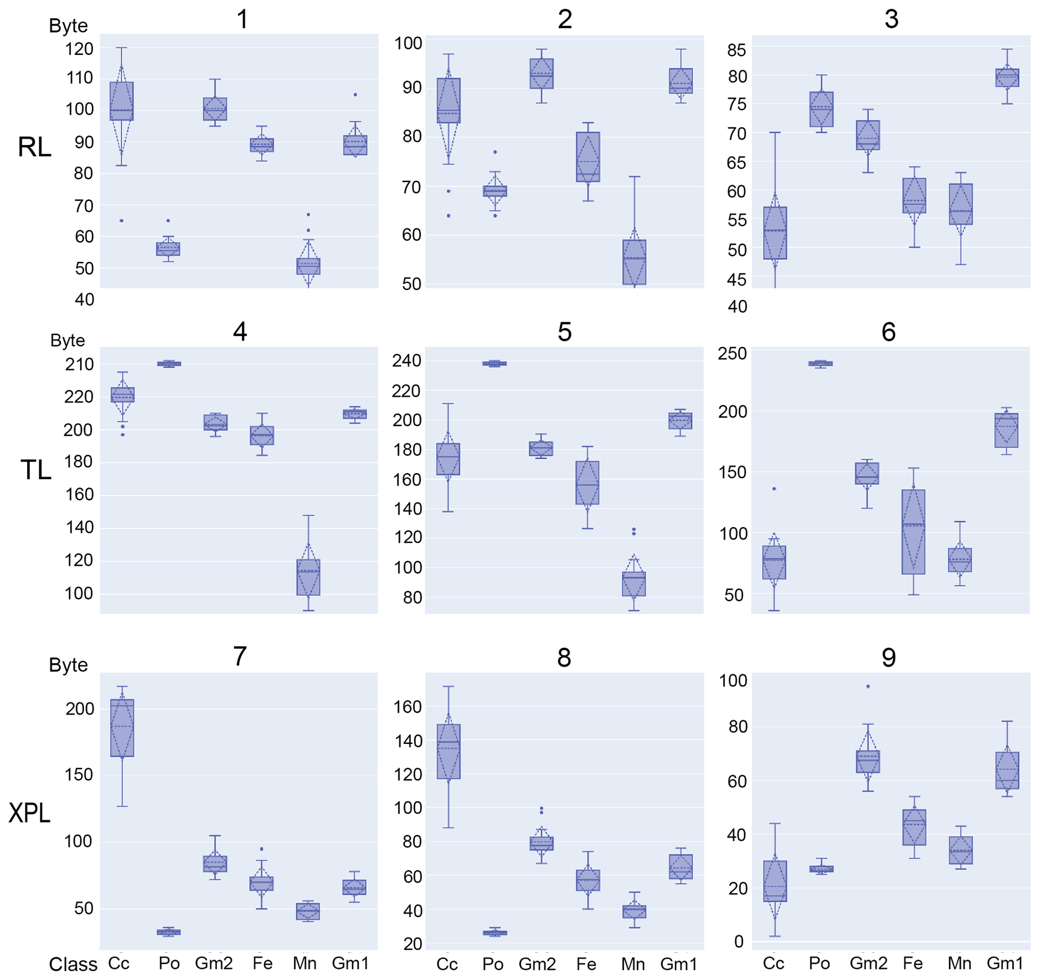
Figure 3MiGIS integrated ROI assessment illustrates training data set validity: class value ranges and standard deviation for each of the RL, TL, and XPL RGB bands 1–9. Data of TS B7 imagery.
2.4.4 Classification, accuracy, and spatial analysis
By running “MiGIS 3 classification”, the classification map (Fig. 1) is generated based on the random forest classification model processed in MiGIS 2.1, and the classification accuracy can be assessed (Sect. 3.1) as an indispensable part of the accuracy assessment (Congalton and Green, 2019). This step requires an independently collected ROI reference data set. In remote sensing analysis this would correspond to ground data (field reference). In MiGIS we use the same vector format ROI data set (Sect. 2.4.2) as for the training. In addition, our reference data sets had the same size as the training data sets to avoid a bias due to different weights. With this second ROI data set, reference values for the individual classes are collected and compared to the classification result. Since our case study was conducted with a modest number of fairly well distinguishable materials and classes, the same processor created the reference data set.
Using the classified and the reference data, a confusion matrix can be calculated and classification accuracy statistics can be derived. The reference data are represented by the columns and the classification result by the rows. Summing all correctly classified pixels (c) divided by the total number of classified pixels (t), the overall accuracy (Eq. 2) indicates the percentage of all pixels that were correctly classified.
For Eqs. (2), (3), and (4), c is sum of all correctly classified pixels, t is total pixel count of classified pixels, cr is correctly classified pixels in reference data (per class), tr is the sum of all classified pixels in reference data (per class), cc is the correctly classified pixel in classified data (per class), and tc is the sum of all classified pixels in classified data (per class).
The producer's accuracy (Eq. 3) indicates what percentage of the respective class areas was correctly identified as such. The user's accuracy (Eq. 4), on the other hand, shows what percentage of the areas assigned to a class is actually part of that class “at ground level” (Congalton and Green, 2019). This allows us to distinguish whether a misclassification (i.e. confusion) occurs due to the training data being inaccurate or because very similar colour properties of two classes evoke increased confusion.
Spatial statistics can be derived from the classification map. If the classification was applied to a cropped image (see Sect. 2.4.1), also the pore space can be quantified. If not, the glass slide rim around the section area would also be included in the pore space's area quantification. Based on the classification map MiGIS 3 calculates feature class-based spatial statistics, which enables the analysis of relative feature quantities in the TS, such as the abundance of a certain feature (e.g. clay coatings). In addition to an output table of pixel areas per class, this can be optionally visualised by running an implemented bar plot function. The classification map itself can be used for further studying distribution patterns in GIS. Classes of interest can be highlighted in colour, whereas other classes can be excluded from the visualisation (see Appendix C1). Such selective visualisations can be used, for example, to illustrate the distribution of diagnostic features. These derivate maps can easily be exported as scaled image files.
The semi-supervised image classification with MiGIS yielded 21 classification maps displaying the distribution of classified features (Sect. 2.1, Table 1) in each TS. Spatial statistics and accuracy assessment results for all TSs of the Rheindahlen sequence are summarised in Appendix B. In Sect. 3.2 we will describe the produced classification maps and spatial statistics of three selected TSs – A4, B7, and C5 (Appendix B) – originating from different Bt horizons of the Rheindahlen sequence (Kehl et al., 2024). This serves to illustrate the classification performance by means of typical micromorphological features, such as pore space (Po), different groundmass types (Gm1/Gm2), quartz sand and gravel grains (Sg), clay coatings (Cc), dark clay coatings (Ccd), iron hydroxide (Fe), and manganese oxides (Mn) pedofeatures. In the following Sect. 3.1, we will describe the methodical outcome (Figs. 4 and 5) and experimental results, conducted to find the most appropriate parameter settings for MiGIS.
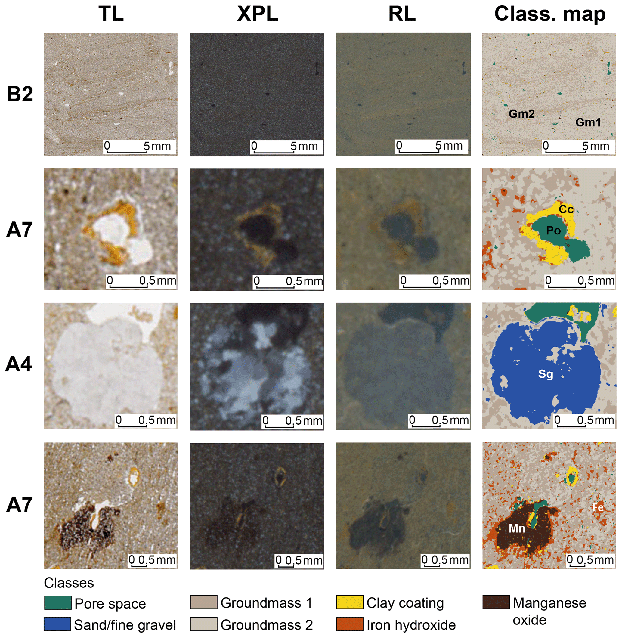
Figure 4Details of selected classification results (Class. map) compared to captures of the transmitted (TL), cross-polarised (XPL), and reflected light (RL) scans of B2: linear basic distribution pattern; A7 (top): clay coating in a vugh; A4: coarse sand grain; A7 (bottom): orthic manganese oxide and iron hydroxide nodule.
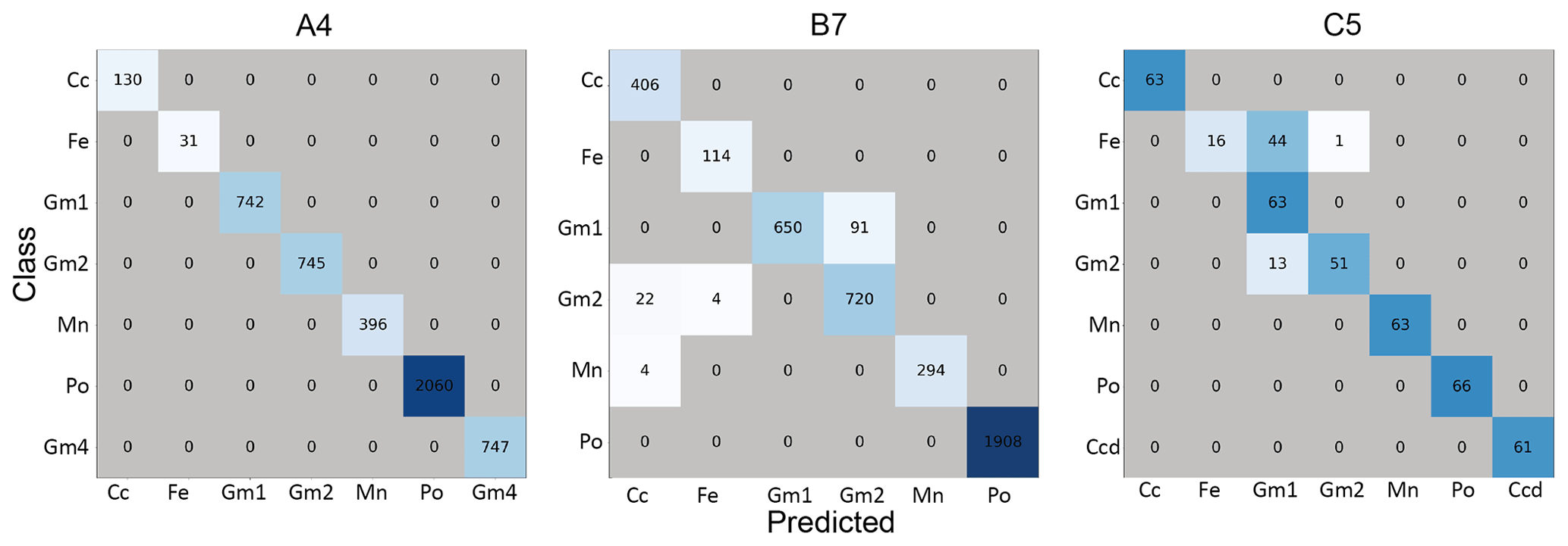
Figure 5Confusion matrices for the classification examples of TS A4 with an overall accuracy of 100 %, B7 with an overall accuracy of 97 %, and C5 with an overall accuracy of 87 %.
3.1 MiGIS classification performance
A detailed examination of Fig. 4 demonstrates that fine linear basic distribution patterns, indicative of disparities in groundmass composition, can be reliably detected, as well as pores, clay coatings, medium to coarse sand and fine gravel grains (quartz), iron hydroxide, and manganese oxide pedofeatures. This outcome underscores the great performance, especially when looking at the clear delimitation of polycrystalline quartz grains from the groundmass and the distinction of finest layer beddings. However, in A7 finer pores are wrongly determined, which may have an influence on the overall porosity; A4 also shows that parts of the sand grain are not recognised, but fine pores are identified as quartz.
Nevertheless, the figure also illustrates the occurrence of misclassifications, especially of fine constituents of the matrix. In the results of TS A7, very fine pores were sometimes classified as groundmass. In A4, however, some small quartz crystals as well as small parts of the larger grain in the middle seem to have been classified as part of the groundmass (Fig. 4).
Examining the classification accuracy (Fig. 5), it must be considered that B7 was one of the first TS data sets to be classified and C5 one of the last. Note that the confusion matrix of B7 has relatively high pixel counts, and that of A4 is medium and that of C5 is relatively low (Fig. 5). This is due to increased confidence in the selection of training and reference data during the test series (Sect. 2.4.2). While the classification of TS A4 achieved an overall accuracy of 100 %, it reaches 97 % accuracy for the classification of TS B7. TS C5 achieves an overall accuracy of only 87 % (Fig. 5 and Appendix B). Comparing all PA values (producer's accuracy) indicates that the classifier exhibited varying accuracy in identifying the targeted feature classes (Appendix B). The same applies for the UA (user's accuracy): the training data accuracy varies between classes. Pore space (Po), medium to coarse sand to fine gravel (Sg), and manganese oxide (Mn) could be identified with a precision of 100 %, whereas Groundmass 1 (Gm1), Groundmass 2 (Gm2), and clay coatings (Cc) indicate confusion in some classification runs: Gm1 only reaches 53 % PA in C5, Gm2 reaches between 98 and 89 % in PA and 97 %–80 % in UA, and the class Cc in B7 achieved only 94 % PA (Appendix B). Apart from this, all PA and UA values for these classes amount to 100 %. Nevertheless, only about half of Gm1 in TS C5 could be correctly identified (Fig. 5). In contrast, the iron-hydroxide-enriched clay coatings (Ccd) in C5 could be identified 100 % of the time. Iron hydroxide (Fe) and class Cc could generally be identified very well, apart from minor confusion regarding Gm2 and Mn in B7. The user's accuracy (UA) assessment indicates a similar pattern to the PA. The classes Po, Sg, and Mn, with a slight variation for Mn in TS B7 (UA: 99 %), are indeed these features as well. Also, in the classes Cc and Ccd, all targeted features can be assigned to the different clay coating types. However, some confusion occurs in the classification of Gm1, Gm2, and Fe in TS B7 and C5. Nevertheless, Fe could also be assigned 100 % of the time in TS A4 and B7. The Fe UA value for TS C5, on the other hand, indicates only a very low accuracy of about 25 % for this class.
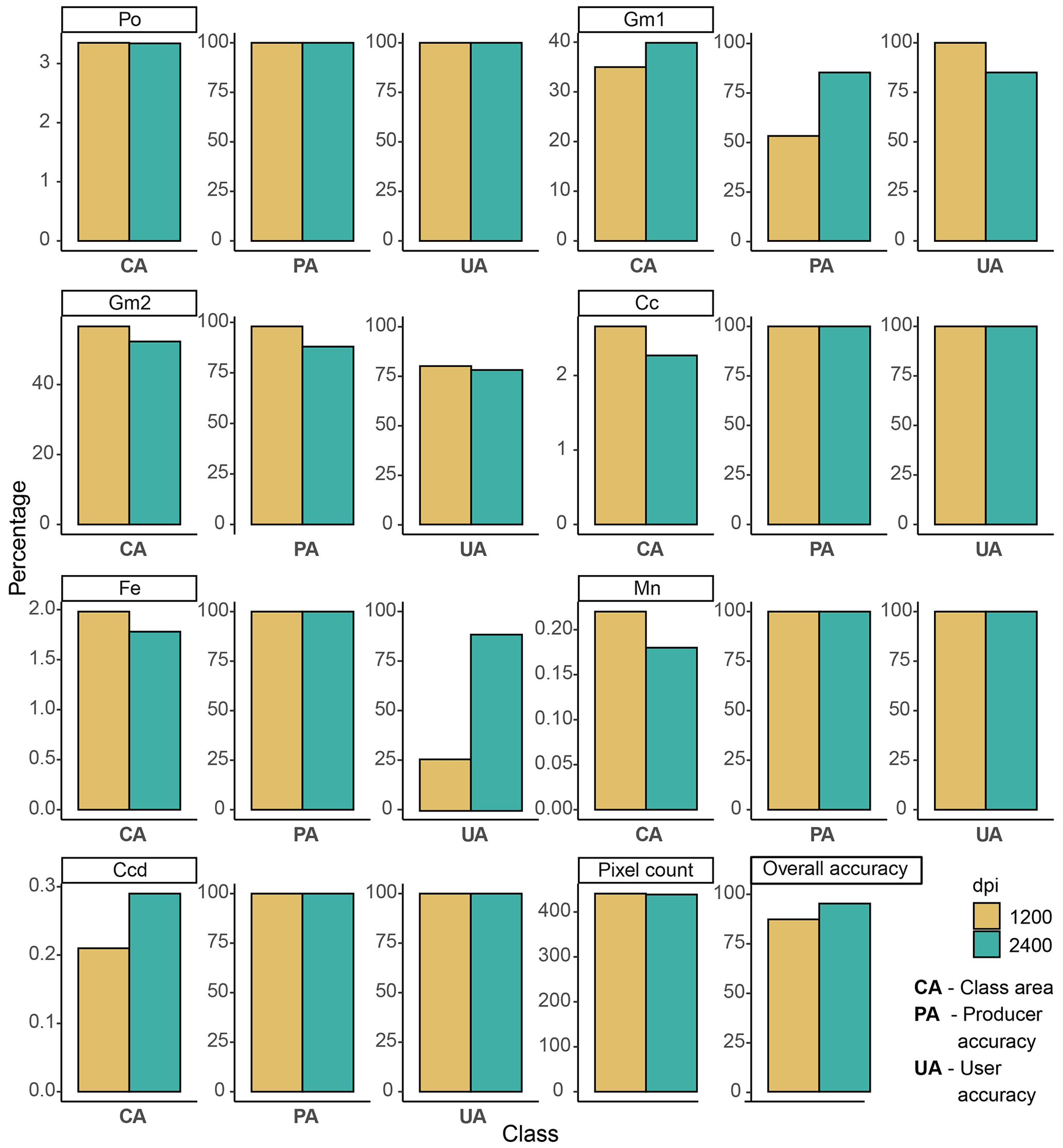
Figure 6Comparison of classified area (CA) proportions and class accuracy parameter (overall, producer's (PA), and user's (UA) accuracy) for thin section (TS) C5, scanned with 1200 and 2400 dpi resolution (data: Appendix B).
A comparison of the classified feature areas and class accuracies of a 1200 dpi and a 2400 dpi scanned data set shows no big differences with regard to the classified feature area. A maximum deviation of 4.8 % in area coverage was observed in class Gm1 (Fig. 6). Indeed, no significant difference in the effective optical image resolution could be observed in direct comparison of the images, whereas there are few discrepancies when comparing the producer's and user's accuracy of the classes.
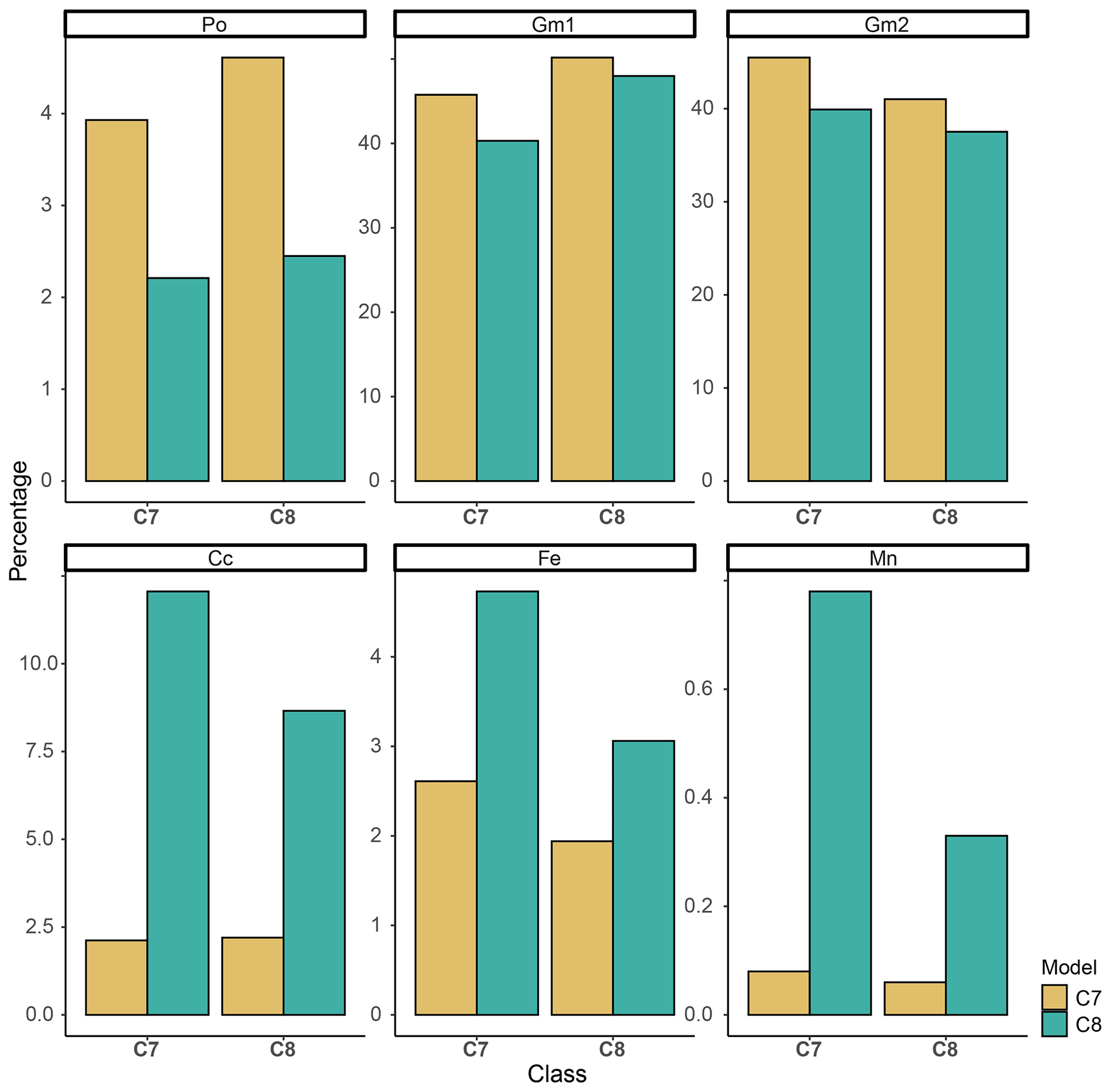
Figure 7Comparison of class area proportions derived from results based on a classification model trained on the same thin section (TS) versus opposite TS. Note the various y-axis scale ranges to ensure the illustration of relative differences within the classes.
We further tested whether a classification model trained on one TS data set can be applied to another data set (Fig. 7).
For this purpose, we selected two TSs with maximum classification “overall accuracy” and a similar composition (i.e. with the same feature classes). The sections C7 and C8 were classified once again with the opposite classification model, and the results were compared. It can be seen that the class areas calculated from these differ significantly in most cases (Fig. 7). This suggests that the classes in the classification models of C7 and C8 are defined by divergent pixel values. Accordingly the multi-RGB signatures differ.
3.2 Digital micromorphological results
All recorded micromorphological features of the different Bt horizons in Rheindahlen are described in detail in Kehl et al. (2024). Here we focus on the micromorphological implications of the classification result. The visual comparison of the classification maps in Fig. 8 facilitates the identification of distinct differences in the microstructure of the selected TSs.
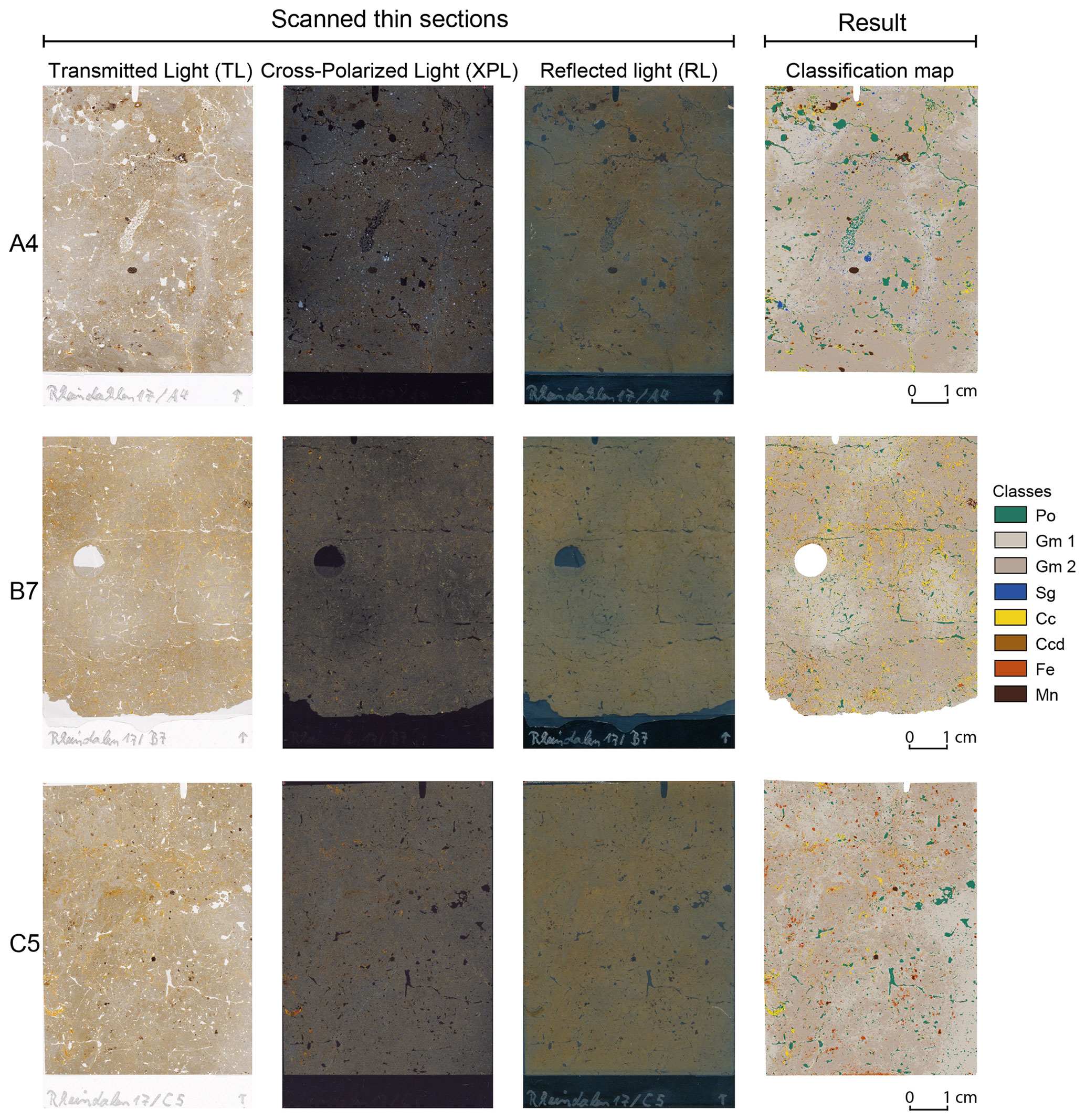
Figure 8Input and output of the image classification of thin section (TS) A4, B7, and C5, which originate from Bt horizons of the Rheindahlen sequence. The classification maps on the right combine the multi-RGB information of the TL, XPL, and RL input images and visualise the spatial distribution patterns of the micromorphological features.
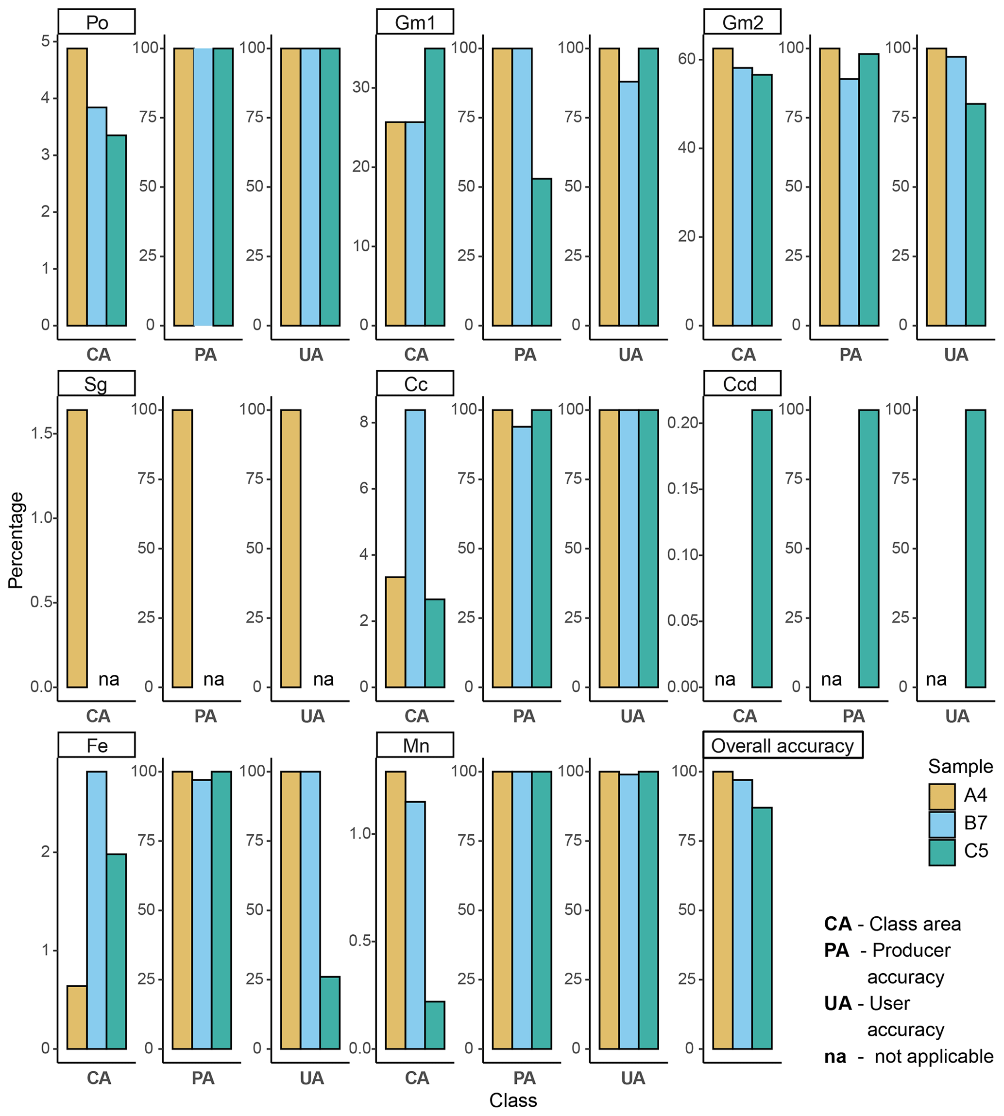
Figure 9Results of the class-based area assessment for thin section A4, B7, and C5. Po: pore space; Gm1: Groundmass 1 (bleached); Gm2: Groundmass 2 (iron hydroxide abundance); Sg: medium and coarse sand and fine gravel; Cc: clay coatings; Ccd: dark clay coatings; Fe: iron hydroxide concretions; Mn: manganese oxide concretions; PA: producer's accuracy; UA: user's accuracy (data: Appendix B).
In A4, vughs, many large channels, and chambers are visible. In contrast, these are smaller and less frequent in B7. Fine planar voids associated with the (sub-)angular blocky microstructure, on the other hand, appear particularly well. These are also found in C5 along with a few channels. In terms of the pore space area, TS B7 and C5 have moderate values between 3.4 % and 2.8 %. In A4, a greater pore space area of 5 % (Po, Fig. 9) indicates increased porosity.
In total five different groundmass types were distinguished in all TSs, and Groundmass 1 (Gm1) and Groundmass 2 (Gm2) are present in the three selected TSs. Qualitative analysis of these two groundmass types indicates that the lighter-coloured (bleached) areas represented by Gm1 are characterised by a decrease in the concentration of iron hydroxide and manganese oxides. In contrast the darker-coloured Gm2 shows an increase in diffusely distributed iron hydroxide. The area ratio of Gm1 and Gm2 is approximately 1 : 2, with values between approximately 25 % (A4 and B7) and 35 % (C5) for Gm1 and values of approximately 57 % (C5), 58 % (B7), and 63 % (A4) for Gm2 (Fig. 9). It demonstrates that the two upper Bt horizons reveal a similar groundmass distribution pattern, whereas the Bt of C5 has a higher fraction of bleached zones. However, the PA score is comparatively low for the class Gm1 in the C5 data set (Fig. 9). The microstructure becomes particularly clear in the separate map representation of the corresponding feature class (Appendix C1). These Bt horizons are characterised by subangular blocky (A4 and B7) to angular blocky or weakly developed platy microstructures (C5), with locally small subangular blocky peds with rounded shapes. The subangular blocky microstructure appears especially well in the classification map of B7 (Fig. 8). Additionally, A4 is one of a few sections of the sequence that contains medium to coarse sand to fine gravel grains whose distribution in the groundmass is visible in the classification map (Fig. 8).
A comparison of all classified pedofeatures indicates distinct spatial distribution patterns, especially when looking at clay coating proportions (Appendix B). These are particularly frequent in Bt horizon TSs from the sequence but are also detected in non-Bt horizons. Mostly they include limpid and occasionally layered slightly impure clay coatings (Cc). They are found in pores, on aggregates, or as fragments (clay papules) in the groundmass. In A4 (3.3 %) and C5 (2.7 %) the proportion is increased. Here mostly intact clay coatings are found, but the amount is low in comparison to the classification results of B7 (8 %). However, the classification map of B7 emphasises a different pattern which links the increased Cc proportion to a high number of clay papules in the matrix.
In contrast, class Ccd, which includes dark clay coatings (enriched with iron hydroxide), is unique for C5 and is represented with 0.2 %. The Fe proportion in C5 is slightly increased (2.0 %), but the manganese oxide proportion is comparatively scarce. However, the UA score is comparatively low for the Fe class (Fig. 9). Even though there is little iron hydroxide in A4, there is a comparatively high proportion of manganese oxide (1.3 %). With an area fraction of 2.8 %, iron hydroxide is very abundant in B7, compared to manganese oxide amounting to 1.2 %.
4.1 Methodological implications of MiGIS
At a first glance, it can be observed that all feature classes can effectively be distinguished by the classifier (Figs. 4, 5, and 9 and Appendix C1). The random forest algorithm proves to be a suitable machine learning method, proficient in handling an expanded number of classes efficiently. Such high class numbers are usually necessary in micromorphology to encompass internal class variations and the irregular occurrence of features in TSs. Rubo et al. (2019) achieved similarly good results when comparing mineralogical and porosity classification model performance of random forest and artificial neural networks. In addition, limiting the trees to a minimum of 100 was considered to fit this variety and proved to perform well (Rubo et al., 2019).
The overall accuracy of the most imprecise classification result of C5, which was 87 %, achieved satisfactory accuracy with regard to established accuracy standards (Anderson et al., 1976). However, in remote sensing analysis, classification results can be affected by atmospheric effects, such as diffuse radiation or clouds, in the input data (Lillesand et al., 2015; Whitcraft et al., 2015). In contrast, we profit from laboratory conditions for the classification of TSs, which increases classification accuracy (Rubo et al., 2019). Nevertheless, a certain “cloudiness” or level of disturbance cannot be neglected. Depending on the TS quality, air bubbles, cracks, etc. influence the classification results.
The classification result details in Fig. 4 illustrate the high accuracy that can be achieved using the random forest algorithm to classify TS scans. By combining the information from three distinct input images (TL, XPL, RL) in the multi-RGB data set, it becomes possible to differentiate features that share similar colour properties in one or even two of the single images. This approach is particularly advantageous when it comes to distinguishing between the Fe and Mn classes. We interpret these classes as predominantly consisting of either iron hydroxides (Fe) or manganese oxides (Mn) (Table 1). Depending on the iron oxide content, both can appear blackish in TL/PPL. Indeed, iron hydroxide has a reddish to brown colour when observed under RL, while manganese oxide appears black as well. The same principle applies to quartz and pore space, which are whitish in TL/PPL, but in XPL quartz shows specific interference colours, and pores are isotropic and hence appear black. (Fig. 4). However, in the case of predominantly occurring fine sand, it is possible that a significant number of the small quartz grains might be oriented in an extinction position without being realised. In this scenario, the probability of confusion with pore space increases due to the overlapping colour values of both entities in XPL. In the RL image, colour distinctions between the two classes are noticeable, likely contributing to the relatively successful classification. Also confusion with the groundmass occurs that is not detected by the accuracy assessment (Fig. 5). This is due to a certain amount of quartz contained in the groundmass. It is conceivable that the classification process might lead to an underestimation of quartz particles in the sand fraction. Consequently, the proportion of sand particles should be considered indicative of minimum values. In contrast, if the interference colours of various occurring mineral grains differ enough, first classification attempts of TS from other sites show that even small mineral grains can be reliably identified. For instance, this applies to carbonates (e.g. limestone) or mica.
Concerning the producer's accuracy, whereas features which are predominantly monochrome (e.g. Po and Mn) reached 100 % identification accuracy, there were minor misclassifications in other classes with increased colour or intensity variation. A confusion of iron hydroxide (Fe) and Groundmass 2 (Gm2) can be related to the fact that iron hydroxide particles are also present in Gm2 (Fig. 4). This illustrates the difficulty of the classifier to properly separate these two classes. Nevertheless, an acceptable classification accuracy of those classes can be yielded, which allows us to estimate the relative distribution of iron hydroxide in the TS.
Regarding the user's accuracy, iron hydroxide could also be assigned 100 % within the classifications of A4 and B7. But the UA for the TS C5, on the other hand, reaches only a very low accuracy of about 25 %. There Fe was largely confused with Gm1, which basically means that some of the created Fe class ROIs must contain pixels that are actually part of the class Gm1. Hence, this training data input should be adjusted.
Initially it is likely that some confusion occurs between feature classes with high similarity in colour such as iron hydroxide and manganese oxides. However, the MiGIS 2.2 tool (Sect. 2.4.3) deals with this issue by visualising the ROI pixel value range per class and band. By a brief examination of the automatically produced boxplot diagrams, it can be investigated whether some ROI positions or their quantity within the respective class would have to be adjusted to improve the classification performance (Sect. 2.4.4). Moreover, it is important to consider all of the presented accuracy assessment parameters (i.e. confusion matrix) when assessing the classification result (Fig. 5).
Smaller particles or pedofeatures, such as thin clay coatings, offer few opportunities for setting sufficient training areas and can therefore also cause misclassifications due to the lack of adequate class size and variation.
In this concern, the application of object-based image analysis (OBIA) instead of colour information classification only could represent a further reasonable adaption, as it combines pixel value classification with segmentation steps (Thierion and Lang, 2018; Visalli et al., 2021). Also, this could be helpful to study geometrical properties of particles, such as single grain rounding and void geometry assessment.
At this stage, we can demonstrate that a classification model trained and applied on an individual TS performs well. However, overfitting can be observed when transferring a created model to another data set. Among others, a successful classification is evoked by representative training data (Vapnik, 2000). Since the colour values of the features between TSs can differ, depending on the type of manufacture, sample, and imagery, the learning of one model might not cover the variation in another TS data set. To avoid model overfitting (Breimann, 2001), more multi-RGB data (i.e. signatures) could be collected from common materials (e.g. features) in TSs. Intensified training on several TS data sets could be a solution to create representative training data to classify TSs produced using a similar resin, technique, and thickness. Such a combined classification model would possibly increase the classification robustness (Breimann, 2001; Vapnik, 2000). In this regard, providing multi-RGB signatures of different features within the application could prove to be supportive for the creation of representative training data. Similar offers exist for remote sensing products, for example provided by the USGS (Kokaly et al., 2017). Nevertheless, the reproducibility of feature signatures based on multi-RGB imagery in terms of increased variation concerning differing colour values between TS images still needs to be investigated. However, our test results (Fig. 7) suggest that great effort is needed to follow this approach, since each TS is a unique product, which implies individual quality characteristics.
In general, a successful classification requires accurately produced TSs. Deviations caused by preparation, such as varying section thickness and embedding resin mixes, air bubbles, and other artefacts, might have a negative effect on the classification result. This is due to the related increased variation in colour of the constituents (i.e. mineral interference colours). Also this limits the transfer of classification models, models which were trained on different TSs (Rubo et al., 2019) and applied to an “untrained” TS data set. Therefore, the application of ML models has so far been broadly limited to the specific TS data set (Sect. 3.1, Fig. 7). At the moment we suggest constructing separate classification models for each thin section.
Apart from preparation quality, classification errors can also be the consequence of discrepancies in the image acquisition (e.g. skewed images, image distortions). For this study, a flatbed scanner with transmitted light imaging was used. This has the advantage that diffuse ambient radiation is greatly minimised by the closed scanner lid. In contrast, such problems can occur when capturing sections with a single-lens reflex (SLR) camera, in addition to an increased probability of distortion due to the curved lens (Carpentier and Vandermeulen, 2016).
Nevertheless, light refraction effects can occur during scanning due to the highly reflective glass slide (Sect. 2.1). At the sample section border they can be excluded during pre-processing in MiGIS 1 (Sect. 2.4.1). Still, light refraction effects can occur at the margins of the pore space. In these transition areas, the embedding resin may not be evenly distributed, which can amplify such effects and consequently cause misclassification. This could possibly be corrected by post-processing through the application of filter algorithms to remove interfering pixel values, for instance by Gaussian smoothing. A similar approach was implemented in the study of Tang et al. (2020).
In general, optical resolution (i.e. spatial resolution) is a limiting factor because this determines the minimum size of detectable micromorphological constituents. The Canon scanner used for this study should be able to produce high-resolution scans of up to 9600 dpi. TS scans of high quality are already obtained at a resolution of 1200 dpi. TS scans taken at 2400 dpi have a higher digital resolution which means that they appear sharper but do not show significantly more detail. Comparing the classification results of both versions the classified feature area differs only minimally (Sect. 3.1, Fig. 6). Thus, the 2400 dpi image does not have a higher spatial resolution. Nevertheless, a direct comparison is difficult because separate training data sets are used for the two image data sets due to the different resolution. This results in the deviations observed in the PA and UA values. However, it is probable that the manufacturer's specification of 9600 dpi refers to the merely maximum possible digital resolution, whereas the maximum optical resolution is 1200 dpi. Furthermore, the pixel values will be interpolated when scanning with a higher-resolution setting than 1200 dpi. This will result in increased file size, and the scanned image appears sharper due to increased digital resolution, but the effective optical resolution remains the same.
Professional film scanners, with a usually much higher optical resolution, can possibly increase the image quality significantly. Thus, approaching the overall resolution limit of 25 µm, especially regarding the fine fraction of the groundmass, all features would appear sharper, and light refraction effects might be minimised. In this regard, it would also be possible to increase the minimum size of observable and analysable constituents, which is 0.1 mm using 1200 dpi scans in this study. However, it must be taken into account that such devices are much more cost intensive than transmitted light flatbed scanners (Haaland et al., 2018).
The total processing (Table 2) time is not constant but is determined, among other things, by the level of experience in creating training areas. In the initial phase of the test series (first TSs classified), the ROIs contained relatively high numbers of pixels (Appendix B). With increasing comprehension of the feature class properties and the algorithm's behaviour, fewer pixels per class were needed to achieve similarly good classification results in later classification runs. Nevertheless, the size of the reference data set used to assess accuracy should correspond to the individual properties (e.g. sample type, resolution, number of classes) of the TS data set (Sect. 2.3). Compared to point counting, which also requires considerably more effort than digital image analysis, it is an advantage that the accuracy does not depend so much on the size of the constituents, as the classification is pixel-based and visual acuity independent (Drees and Ransom, 1994; Murphy et al., 1977).
4.2 Interpretation of the digital micromorphological results
Though an exhaustive interpretation of sediment and soil formation processes at Rheindahlen exceeds the confines of this paper, we aim to provide illustrative examples of how the derived proportions and distribution patterns of classified constituents can augment the comprehension of conventional micromorphological analyses and to improve the dissemination of the findings.
The visualised microstructure and the determined porosity values (Sect. 3.2) can be well assigned to the Bt horizon spectrum (Kehl et al., 2024). Compared to most other samples, the bleached Groundmass 1 (Gm1) is less represented in all analysed TSs, whereas Groundmass 2 (Gm2), characterised by evenly distributed and stronger iron staining, is much more represented. Gm1 identifies parts where iron hydroxide is lacking due to redoximorphic bleaching. This can be easily brought into proportion through the classification and enables an estimation of the relative iron hydroxide content and depletion rates under the assumption that Gm2 represents the pre-depletion state (Sect. 3.2 and Kehl et al., 2024).
The uppermost part of the studied profile, including the modern Bt horizon represented by TS A4, contains a notable amount of medium to coarse sand and fine gravel. In silt-dominated loess deposits, inclusion of such grains indicates reworking of the aeolian deposit by overland flow or solifluction. In addition, the patchy distribution pattern of such grains in thin section A7 can be linked to cryoturbation processes (Kehl et al., 2024).
In all presented TSs of the Bt horizons many well-developed clay coatings are preserved (Fig. 9), especially in large pores. B7 has the highest proportion of clay coatings in the entire sequence, indicating a particularly intensive and long-term character of soil formation during the related interglacial period (Kehl et al., 2024). The clay coatings of the lower Bt horizons displayed in B7 and C5 are often fragmented, and clay papules are abundant (Sect. 3.2). Frost effects are attributed to this mechanical disruption of clay coatings, a phenomenon not observed in the modern Bt horizon of A4.
The abundance of redoximorphic pedofeatures in TS A4 is particularly well displayed in the respective single maps (Appendix C1). In general, these features indicate the effect of stagnant water conditions. In the presented TSs, they are less than 1 mm in diameter, but also some larger nodules, measuring more than 5 mm, have been observed in some parts, such as in TS A4. However, especially in thin section C5, the increased number of iron hydroxide and manganese oxide nodules, microscopically determined in the lower part of the sequence (TS C5–C8; Kehl et al., 2024), are not reflected by the classification results. This could be partly attributed to the classification method, which quantifies the aerial percentage of nodules rather than their numerical count.
Nevertheless, the increased confusion with class Gm2, which contains fine-grained iron hydroxide, accompanied by the low UA score, seems to have led to the underestimation of the corresponding classes Fe and Mn (Appendix B).
4.3 Implications for micromorphology
The employment of MiGIS as an auxiliary instrument reveals its efficacy in mapping and quantifying soil and sediment constituents based on their multi-RGB signature (Fig. 2), thereby demonstrating the advantageous integration of this supplementary digital dimension into micromorphological analysis. Nevertheless, the MiGIS classification using the random forest algorithm is based on colour values (TL, XPL, and RL) of the TS features. A classification based on shape and size is not included yet. This could possibly be implemented by using OBIA algorithms through the process of image segmentation (Sect. 4.1).
However, the semi-automatic classification approach of MiGIS enables users, e.g. well-trained micromorphologists, to define suitable training data for specific feature classes. This offers the advantages of qualitative control concerning TS imagery, as well as a suitability assessment of colour value differences between constituents. The application of a mask layer to crop the multi-band layer, which is used to select the classification area (sample section) in MiGIS 1, also enables the definition of relevant parts of the sample. Thus, artefact sections such as drying cracks can be excluded. Comparatively fast digital documentation within 1.5–2.5 h processing time (software familiarisation inclusive) per TS enables a straightforward assessment of the overall composition, pore space volume, distribution patterns, and microstructure, in combination with an automated visualisation of these results. Trends and anomalies can thus be highlighted (e.g. by setting a high-contrast colour for a specific feature class), and at the same time feature occurrence can be recorded for statistics without much effort. By classifying entire TSs, feature quantities and spatial patterns can be compared between different TSs (i.e. stratigraphical units). This is of minor interest in digital petrographic analyses, which is mostly focused on the classification of microphotographs (Ghiasi-Freez et al., 2012; Naseri and Rezaei Nasab, 2021; Rubo et al., 2019; Tang et al., 2020), but very innovative for micromorphological analyses. Nevertheless, MiGIS can also be used for the classification of microphotographs. Moreover, it would be conceivable to use the method to verify sedimentological anomalies, for instance, to identify a weakly expressed archaeological context or feature. Within our working group, MiGIS has already been tested on TSs from archaeological sediments. Even though the material diversity can be significantly higher due to anthropogenic input, the first promising results have already been achieved, e.g. for cave occupation layers and floor contexts in tell sediments. Thus, we plan to evaluate the application of MiGIS to archaeological TSs.
Similar to the studies of Tarquini and Favalli (2010) and Visalli et al. (2021), the GIS environment, which was applied here, is advantageous to survey and query the TS imagery and the classification map within a metric spatial reference system. Thus, realistic spatial measurements, provided by the use of a metric CRS (Sect. 2.2), allow native QGIS measurement and spatial analysis tools (QGIS Development Team, 2022b) to be used to capture the dimensions or distribution of micromorphological features. In addition, vectorisation in post-processing of the classification maps enables the use of geometric analysis and further query tools (Visalli et al., 2021). In this sense, the combination of mapping and quantification of constituents in TSs can be gainfully applied for micromorphological analysis and documentation.
However, there are some limitations regarding the significance of measurement results and quantification. Still, a proper classification requires expert microscopic analysis, specifically to assess the individual use of principally underestimated pore space quantification which is obtained by the digital classification approach (Sect. 2.1). Nevertheless, by classifying the pore space of an entire TS, the microstructure can be visualised to a high degree of effectiveness. The classification of the groundmass is also an advantage for capturing the respective spatial composition. For instance, this enables the recognition and illustration of bedding features or linear basic distribution patterns, as well as the degree of soil formation (Sect. 3.1, Fig. 4).
Also, improvements could be made with regard to the misclassifications of manganese oxides and iron hydroxide. Our approach is based on the classification of colour values only, but these can vary not only due to the TS quality, but also in the case of manganese and iron oxide concretions due to the presence of other chemical elements such as phosphorus (Vepraskas et al., 2018). Accordingly, a precise micromorphological analysis is always a prerequisite for the digital analysis, although, referring to Rubo et al. (2019), using chemical or element mapping imagery (micro-XRF) as additional input to improve the classification could be very useful in this concern (Mentzer, 2017; Visalli et al., 2021). Comparing MiGIS classification to element mappings could also provide an independent, detailed compositional reference. For instance, element maps could be used to verify the spatial distribution of specific elements, such as Fe or Mn.
We presented the freely accessible MiGIS toolbox, an innovative tool for digital micromorphological TS analysis based on multi-RGB TS imagery. It can be applied by integrating Python processing scripts (“Code and data availability” section) into the open-source software QGIS 3. The application of a metric CRS enables realistic measurements based on scanned TL, XPL, and RL imagery. The ability to classify TS features using their colour value signature, quantify them, and visualise spatial relationships makes MiGIS a useful supplement to conventional micromorphological analysis (Sect. 4.3).
In particular, the visualisation of the spatial distribution of pedofeatures and their quantification could be profitably used for the determination of Bt horizons from the Rheindahlen loess–palaeosol sequence. In this way micromorphological observations become vivid and to a certain extent reproducible. Moreover, the computed spatial statistics enable the quantification of observations (i.e. features) to compare the composition and structure of different samples. Likewise, this could prove to be useful for pedological, sedimentological, and microfacies analyses. However, the achieved classification accuracy depends on the user's academic training level (i.e. in micromorphology or petrography) and the ability to create representative training data. Thus, basic knowledge of the principles of ML-based image classification and GIS functionalities in general are indispensable. Nevertheless, implemented control instances, such as pre-classification ROI evaluation (Sect. 2.4.3) and using a set of independent ROIs for reference, allow for a certain self-control. Further it turned out that a scan resolution of 1200 dpi is sufficient to produce suitable classification results. Also, the random forest algorithm seems to be well-suited for the semi-supervised classification of typically high colour value variation in TS features and high number of classes (Sect. 4.2).
The application of element maps (micro-XRF) could serve as a further reference but could also boost the classification accuracy especially of Fe and Mn features (Sect. 4.1). Even involving several feature classes (Table 1), it turns out that the obtained classification results of a model trained and applied on the same TS are reliable. Nevertheless, the efficiency could still be increased by creating a combined classification model and applying it for a whole sequence, or for micromorphological features in general. Considerable effort is required to establish a comprehensive signature library for micromorphological features in multi-RGB imagery, taking into account the influence of variable TS quality and recording modes as limiting factors. Moreover, a preliminary investigation is essential to determine the reproducibility of multi-RGB signatures for individual features (Sect. 4.1). Implementing an OBIA function in individual classification runs could provide the classification result with further detail, for example to differentiate between geometrical properties of features (Sect. 4.1). In general, since MiGIS is based on a Python script, a reasonable next step will be the implementation as an official plugin in the QGIS repository, which would increase accessibility.
Table A1Implemented geoalgorithms in MiGIS toolbox with references.
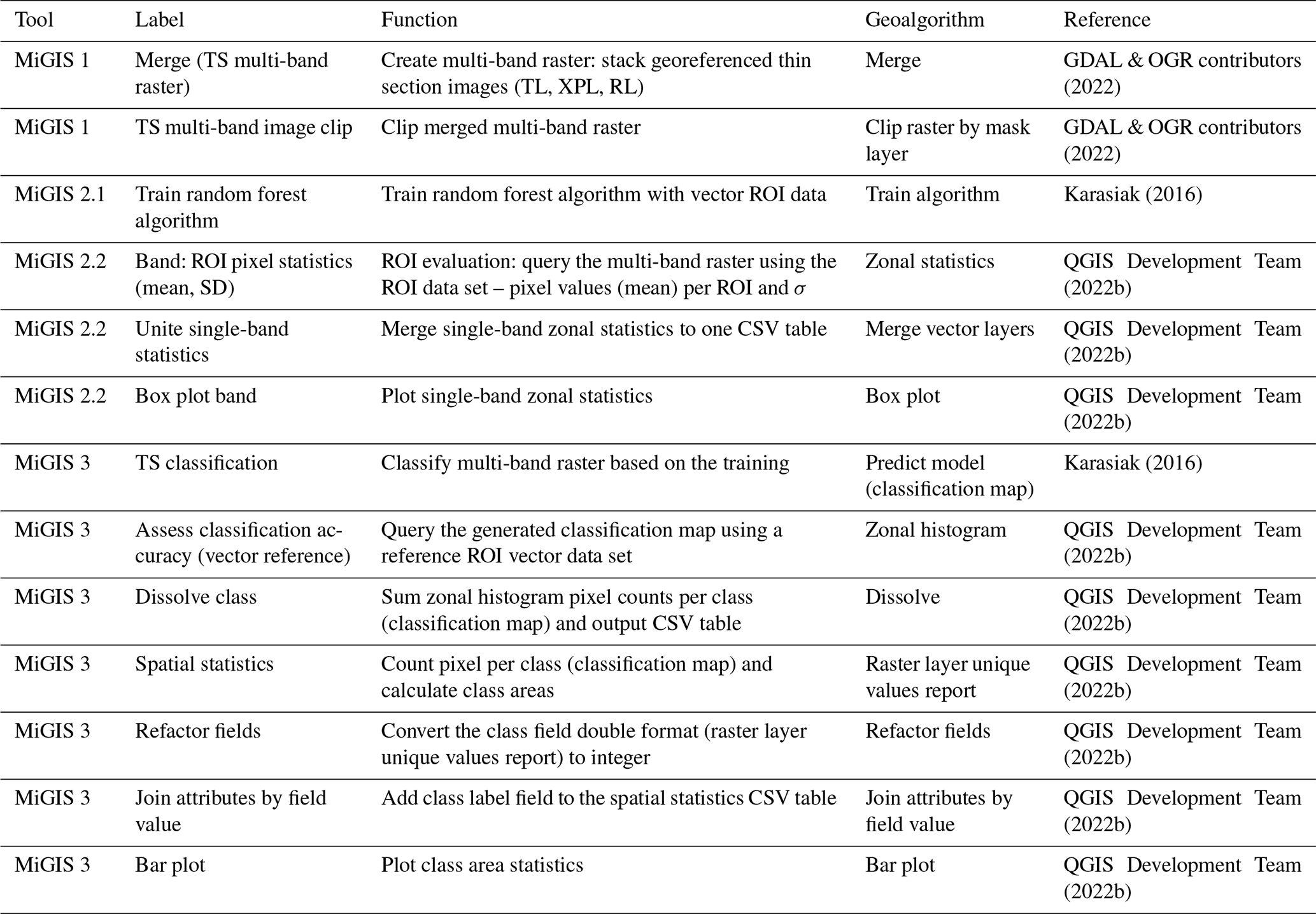
Table B1Total thin section (TS) classification results for the Rheindahlen stratigraphy. TS image classifications presented in Sect. 3 are highlighted. OA: overall accuracy; PA: producer's accuracy; UA: user's accuracy; n/a: respective constituent (feature class) not present in the TS. Quality criteria: 100 %–90 % class accuracy – very good; ∗ 90 %–80 % class accuracy – good; < 80 % class accuracy – poor.
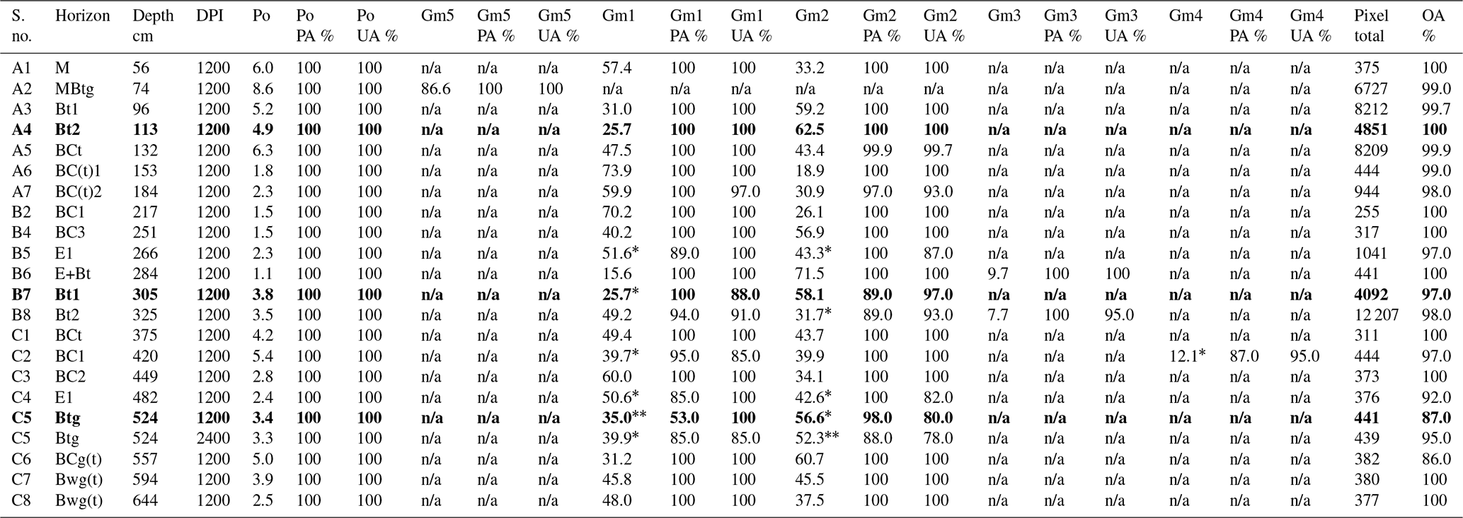
Table B2Total thin section (TS) classification results for the Rheindahlen stratigraphy. TS image classifications presented in Sect. 3 are highlighted. OA: overall accuracy; PA: producer's accuracy; UA: user's accuracy; n/a: respective constituent (feature class) not present in the TS. Quality criteria: 100 %–90 % class accuracy – very good; ∗ 90 %–80 % class accuracy – good; < 80 % class accuracy – poor.
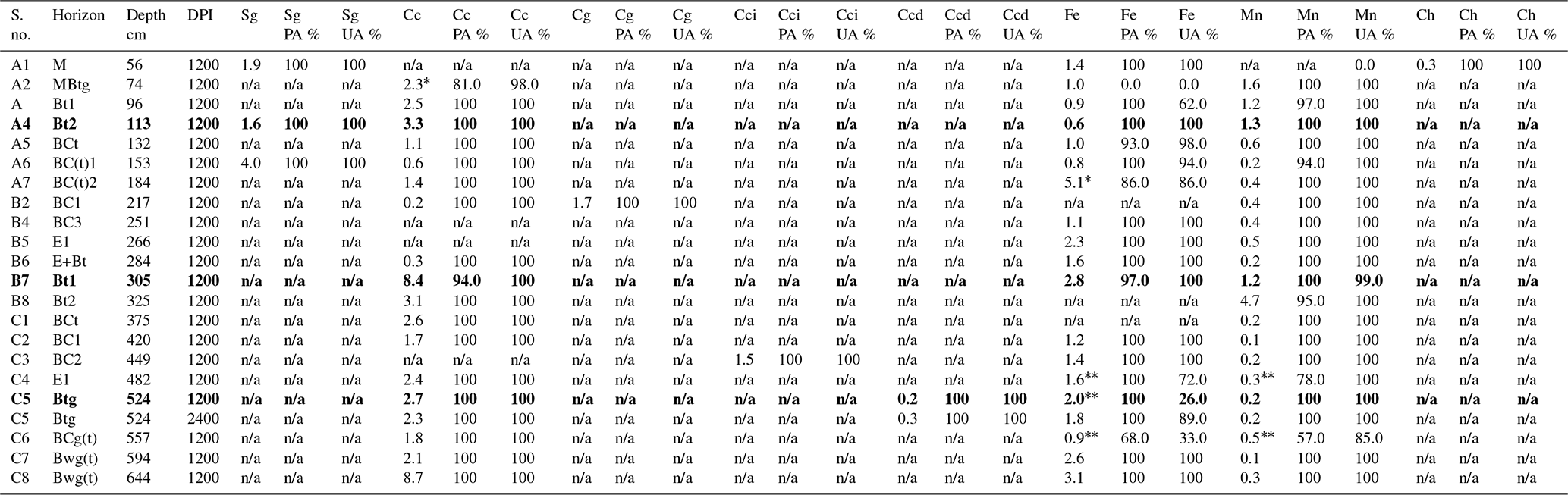
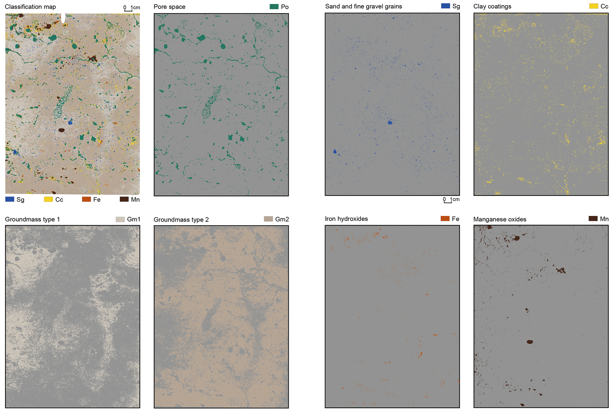
Figure C1Individual visualisation of classified feature classes, derived from the classification map of thin section (TS) A4.
All MiGIS toolbox Python processing scripts for QGIS 3 – MiGIS 1 preprocess TS images, MiGIS 2.1 train algorithm, MiGIS 2.2 ROI evaluation (optional), MiGIS 3 classification – and templates are freely available online on GitHub: https://github.com/Mirijamz/MiGIS (last access: 18 January 2024; https://doi.org/10.5281/zenodo.10527165, Zickel and Gröbner, 2023). In addition to tool scripts and template files, an accompanying toolbox manual (documentation) is available at the above address on GitHub. MiGIS toolbox is based on open-source resources provided by GDAL, Nicolas Karasiak, QGIS, and the Scikit-learn developers. Accordingly, software and underlying code are available on GitHub and Zenodo: GDAL v3.5.1 from https://github.com/OSGeo/gdal (last access: 24 January 2024; https://doi.org/10.5281/zenodo.6801315, Rouault et al., 2022); Dzetsaka Qgis Classification plugin v3.7 from https://github.com/nkarasiak/dzetsaka/ (last access: 24 January 2024; https://doi.org/10.5281/zenodo.3463523, Karasiak, 2019); QGIS v3.22 from https://github.com/qgis/QGIS (last access: 24 January 2024; https://doi.org/10.5281/zenodo.7986774, qgis bot., 2022); and scikit-learn v1.0.1 from https://github.com/scikit-learn/ (last access: 24 January 2024; https://doi.org/10.5281/zenodo.5596244, Grisel et al., 2021).
MK provided the resources and supervised the project. MZ did conceptualisation and developed the methodology and the code. MG mainly did the data acquisition and curation. MZ, MG, and MK were engaged in the investigation. MZ did the formal analysis, worked on the visualisation of the results together with MG, and prepared the original draft. AR and MK validated the results. MZ, MG, AR, and MK did the writing, review, and editing.
The contact author has declared that none of the authors has any competing interests.
Publisher's note: Copernicus Publications remains neutral with regard to jurisdictional claims made in the text, published maps, institutional affiliations, or any other geographical representation in this paper. While Copernicus Publications makes every effort to include appropriate place names, the final responsibility lies with the authors.
We express our gratitude for the financial backing extended through grant number 408333614 and the coverage of the article processing charge (grant no. 491454339) by the German Research Foundation (DFG). The authors wish to convey their appreciation to Tony Reimann, Stephan Opitz, and Christoph Hütt for their insightful discussions on the results and their assistance in crafting and refining the article. Additionally, we extend our thanks to the reviewers whose valuable comments and guidance substantially enhanced the quality of this paper.
This research has been supported by the Deutsche Forschungsgemeinschaft (grant nos. 408333614 and 491454339).
This open-access publication was funded by Universität zu Köln.
This paper was edited by Christian Zeeden and reviewed by David Brönnimann and Janek Walk.
Anderson, J. R., Hardy, E. E., Roach, J. T., and Witmer, R. E.: A land use and land cover classification system for use with remote sensor data, Tech. rep., USGS Publications Warehouse, Professional Paper, 964, Reston, USA, https://doi.org/10.3133/pp964, 1976. a
Arnay, R., Hernández-Aceituno, J., and Mallol, C.: Soil micromorphological image classification using deep learning: The porosity parameter, Appl. Soft Comput., 102, 107093, https://doi.org/10.1016/j.asoc.2021.107093, 2021. a
Arpin, T. L., Mallol, C., and Goldberg, P.: Short contribution: A new method of analyzing and documenting micromorphological thin sections using flatbed scanners: Applications in geoarchaeological studies, Geoarchaeology, 17, 305–313, https://doi.org/10.1002/gea.10014, 2002. a, b
Beckmann, T.: Präparation bodenkundlicher Dünnschliffe für mikromorphologische Untersuchungen, Hohenheimer Bodenkundliche Hefte, 40, 89–103, 1997. a
Breimann, L.: Random Forests, Mach. Learn., 45, 5–32, https://doi.org/10.1023/A:1010933404324, 2001. a, b, c, d
Brewer, R.: Fabric and mineral analysis of soils, John Wiley & Sons, New York, USA, 1964. a
Brönnimann, D., Röder, B., Spichtig, N., Rissanen, H., Lassau, G., and Rentzel, P.: The Hidden Midden: Geoarchaeological investigation of sedimentation processes, waste disposal practices, and resource management at the La Tène settlement of Basel-Gasfabrik (Switzerland), Geoarchaeology, 35, 522–544, https://doi.org/10.1002/gea.21787, 2020. a
Bullock, P. and International Society of Soil Science: Handbook for Soil Thin Section Description, Waine Research, Albrighton, UK, 1985. a, b
Canti, M. and Huisman, D. J.: Scientific advances in geoarchaeology during the last twenty years, J. Archaeol. Sci., 56, 96–108, https://doi.org/10.1016/j.jas.2015.02.024, 2015. a
Carpentier, F. and Vandermeulen, B.: High-Resolution Photography for Soil Micromorphology Slide Documentation, Geoarchaeology, 31, 603–607, https://doi.org/10.1002/gea.21563, 2016. a
Congalton, R. G. and Green, K.: Assessing the Accuracy of Remotely Sensed Data – Principles and Practices Third edition, CRC Press, Taylor & Francis Group, Boca Raton, USA, 3rd edn., ISBN 978-1-4200-5512-2, https://doi.org/10.1201/9780429052729, 2019. a, b
Courty, M. A., Goldberg, P., and MacPhail, R. I.: Soils and Micromorphology in Archaeology, Cambridge University Press, Cambridge, UK, ISBN 9780521324199, 1989. a
Drees, L. R. and Ransom, M. D.: Light Microscopic Techniques, in: Quantitative Methods in Soil Mineralogy, edited by: Chair, J. E. A. and Stucki, J. W., chap. 5, John Wiley & Sons, Ltd, ISBN 9780891188841, 137–176, https://doi.org/10.2136/1994.quantitativemethods.c5, 1994. a, b, c
FitzPatrick, E. A.: Micromorphology of Soils, Springer Science & Business Media, London, 2nd edn., ISBN 9789400955448 , 2012. a, b, c
GDAL & OGR contributors: GDAL & OGR Geospatial Data Abstraction software Library, release 3, https://gdal.org/ (last access: 18 January 2024), 2022. a, b, c
Ghiasi-Freez, J., Soleimanpour, I., Kadkhodaie-Ilkhchi, A., Ziaii, M., Sedighi, M., and Hatampour, A.: Semi-automated porosity identification from thin section images using image analysis and intelligent discriminant classifiers, Comput. Geosci., 45, 36–45, https://doi.org/10.1016/j.cageo.2012.03.006, 2012. a, b
Grisel, O., Mueller, A., Gramfort, L. A., Louppe, G., Prettenhofer, P., Blondel, M., Niculae, V., Nothman, J., Joly, A., Fan, T. J., Vanderplas, J., Kumar, M., Lemaitre, G., Qin, H., Hug, N., Estève, L., Varoquaux, N., Layton, R., Metzen, J. H., Jalali, A., (Venkat) Raghav, R., Schönberger, J., du Boisberranger, J., Yurchak, R., Li, W., la Tour, T. D., Woolam, C., Eren, K. and Diemert, E.: scikit-learn/scikit-learn: scikit-learn 1.0.1, version 1.0.0, Zenodo [code], https://doi.org/10.5281/zenodo.5596244, 2021. a
Haaland, M. M., Czechowski, M., Carpentier, F., Lejay, M., and Vandermeulen, B.: Documenting archaeological thin sections in high-resolution: A comparison of methods and discussion of applications, Geoarchaeology, 34, 100–114, https://doi.org/10.1002/gea.21706, 2018. a, b, c
IUSS Working Group (WRB): World Reference Base for Soil Resources. International soil classification system for naming soils and creating legends for soil maps, 4th edn., International Union of Soil Sciences (IUSS), Vienna, Austria, ISBN 9798986245119, 2022. a
Karasiak, N.: Dzetsaka Qgis Classification plugin, version 3.7, Zenodo [code], https://doi.org/10.5281/zenodo.2552284, 2016. a, b, c, d, e
Karasiak, N.: lennepkade/dzetsaka: Fix bug in processing provider with vector files (Dzetsaka QGIS classification plugin), version 3.5.1, Zenodo [code], https://doi.org/10.5281/zenodo.3463523, 2019. a
Kehl, M., Seeger, K., Pötter, S., Schulte, P., Klasen, N., Zickel, M., Pastoors, A., and Claßen, E.: Loess formation and chronology at the Palaeolithic key site Rheindahlen, Lower Rhine Embayment, Germany, E&G Quaternary Sci. J., 73, 41–67, https://doi.org/10.5194/egqsj-73-41-2024, 2024. a, b, c, d, e, f, g, h, i, j, k, l
Kokaly, R. F., Clark, R. N., Swayze, G. A., Livo, K. E., Hoefen, T. M., Pearson, N. C., Wise, R. A., Benzel, W., Lowers, H. A., Driscoll, R. L., and Klein, A. J.: USGS Spectral Library Version 7, Data series 1035, U.S. Geological Survey, Reston, USA, https://doi.org/10.3133/ds1035, 2017. a
Ligouis, B.: Reflected Light, in: Archaeological Soil and Sediment Micromorphology, edited by: Nicosia, C. and Stoops, G., chap. 44, John Wiley & Sons, Ltd, ISBN 9781118941065, 461–470, https://doi.org/10.1002/9781118941065.ch44, 2017. a
Lillesand, T., Kiefer, R., and Chipman, J.: Remote Sensing and Image Interpretation, 7th edn., John Wiley & Sons, Ltd., New York, USA, ISBN 9781118343289, 2015. a, b, c
Lo Russo, S., Brönnimann, D., Deschler-Erb, S., Ebnöther, C., and Rentzel, P.: Mithraism under the microscope:: new revelations about rituals through micromorphology, histotaphonomy and zooarchaeology, Archaeol. Anthrop. Sci., 14, 1–21, https://doi.org/10.1007/s12520-022-01505-6, 2022. a
Mentzer, S. M.: Micro XRF, in: Archaeological Soil and Sediment Micromorphology, edited by: Nicosia, C. and Stoops, G., chap. 41, John Wiley & Sons, Ltd, ISBN 9781118941065, 431–440, https://doi.org/10.1002/9781118941065.ch41, 2017. a
Murphy, C. P., Bullock, P., and Turner, R. H.: The Measurement And Characterisation Of Voids In Soil Thin Sections By Image Analysis. Part I. Principles And Techniques, J. Soil Sci., 28, 498–508, https://doi.org/10.1111/j.1365-2389.1977.tb02258.x, 1977. a, b
Naseri, A. and Rezaei Nasab, A.: Automatic identification of minerals in thin sections using image processing, J. Amb. Intel. Hum. Comp., 14, 3369–3381, https://doi.org/10.1007/s12652-021-03474-5, 2021. a, b
Nesse, W.: Introduction to Optical Mineralogy, Oxford University Press, ISBN 9780199846276, 2013. a
Nicosia, C. and Stoops, G. (Eds.): Archaeological Soil and Sediment Micromorphology, John Wiley, Chichester, UK, https://doi.org/10.1002/9781118941065, 2017. a
Pedregosa, F., Varoquaux, G., Gramfort, A., Michel, V., Thirion, B., Grisel, O., Blondel, M., Prettenhofer, P., Weiss, R., Dubourg, V., Vanderplas, J., Passos, A., Cournapeau, D., Brucher, M., Perrot, M., and Édouard Duchesnay: Scikit-learn: Machine Learning in Python, J. Mach. Learn. Res., 12, 2825–2830, http://jmlr.org/papers/v12/pedregosa11a.html (last access: 18 January 2024), 2011. a, b
Pires de Lima, R., Duarte, D., Nicholson, C., Slatt, R., and Marfurt, K. J.: Petrographic microfacies classification with deep convolutional neural networks, Comp. Geosci., 142, 104481, https://doi.org/10.1016/j.cageo.2020.104481, 2020. a
qgis-bot.: qgis/QGIS: 3.22.10 (final-3_22_10), version 3.22, Zenodo [code], https://doi.org/10.5281/zenodo.7986774, 2022.
QGIS Development Team: QGIS Geographic Information System software, version 3.22, Open Source Geospatial Foundation Project [code], http://qgis.org (last access: 18 January 2024), 2022a. a, b
QGIS Development Team: Documentation for QGIS 3.22, QGIS – Geographic Information System, QGIS Association, https://docs.qgis.org/3.22/en/docs/ (last access: 18 January 2024), 2022b. a, b, c, d, e, f, g, h, i, j, k, l
Rouault, E., Warmerdam, F., Schwehr, K., Kiselev, A., Butler, H., Łoskot, M., Szekeres, T., Tourigny, E., Landa, M., Miara, I., Elliston, B., Kumar, C., Plesea, L., Morissette, D., Jolma, A., and Dawson, N.: GDAL, version 3.5.1, Zenodo [code], https://doi.org/10.5281/zenodo.6801315, 2022. a
Rubo, R. A., de Carvalho Carneiro, C., Michelon, M. F., and dos Santos Gioria, R.: Digital petrography: Mineralogy and porosity identification using machine learning algorithms in petrographic thin section images, J. Petrol. Sci. Eng., 183, 106382, https://doi.org/10.1016/j.petrol.2019.106382, 2019. a, b, c, d, e, f, g, h
Sauzet, O., Cammas, C., Gilliot, J. M., Bajard, M., and Montagne, D.: Development of a novel image analysis procedure to quantify biological porosity and illuvial clay in large soil thin sections, Geoderma, 292, 135–148, https://doi.org/10.1016/j.geoderma.2017.01.004, 2017. a
Scikit-learn developers: User guide: 1.11.2. Forests of randomized trees, Scikit-learn community, https://scikit-learn.org/stable/modules/ensemble.html#random-forests (last access: 18 January), 2007–2023. a, b
Shahack-Gross, R.: Archaeological Micromorphology Self-Evaluation Exercise, Geoarchaeology, 31, 49–57, https://doi.org/10.1002/gea.21536, 2015. a
Stoops, G.: Guidelines for Analysis and Description of Soil and Regolith Thin Sections, ASA, CSSA, and SSSA books, Soil Science Society of America, Inc., Wiley (online), 2nd edn., https://doi.org/10.1002/9780891189763, 2020. a, b, c, d, e, f, g, h
Stoops, G., Marcelino, V., and Mees, F. (Eds.): Interpretation of Micromorphological Features of Soils and Regoliths, 2nd edn., Elsevier, ISBN 978-0-444-63522-8, https://doi.org/10.1016/C2014-0-01728-5, 2018. a, b, c
Tang, D. G., Milliken, K. L., and Spikes, K. T.: Machine learning for point counting and segmentation of arenite in thin section, Mar. Petrol. Geol., 120, 104518, https://doi.org/10.1016/j.marpetgeo.2020.104518, 2020. a, b, c, d
Tarquini, S. and Favalli, M.: A microscopic information system (MIS) for petrographic analysis, Comput. Geosci., 36, 665–674, https://doi.org/10.1016/j.cageo.2009.09.017, 2010. a, b, c
Thierion, V. and Lang, M.: Object-Based Classification for Mountainous Vegetation Physiognomy Mapping, in: QGIS and Applications in Agriculture and Forest, edited by: Baghdadi, N., Mallet, C., and Zribi, M., chap. 9, John Wiley & Sons, Ltd, ISBN 9781119457107, 283–339, https://doi.org/10.1002/9781119457107.ch9, 2018. a
van der Meer, J. J. M. and Menzies, J.: The micromorphology of unconsolidated sediments, Sediment. Geol., 238, 213–232, 2011. a
Vapnik, V. N.: The Nature of Statistical Learning Theory, Springer New York, New York, USA, ISBN 978-1-4757-3264-1, https://doi.org/10.1007/978-1-4757-3264-1, 2000. a, b
Vepraskas, M. J., Lindbo, D. L., and Stolt, M. H.: Redoximorphic Features, in: Interpretation of Micromorphological Features of Soils and Regoliths (Second Edition), edited by: Stoops, G., Marcelino, V., and Mees, F., Elsevier, 425–445, https://doi.org/10.1016/b978-0-444-63522-8.00015-2, 2018. a, b
Visalli, R., Ortolano, G., Godard, G., and Cirrincione, R.: Micro-Fabric Analyzer (MFA): A New Semiautomated ArcGIS-Based Edge Detector for Quantitative Microstructural Analysis of Rock Thin-Sections, ISPRS Int. J. Geo-Inf., 10, 51, https://doi.org/10.3390/ijgi10020051, 2021. a, b, c, d, e
Whitcraft, A., Vermote, E. F., Becker-Reshef, I., and Justice, C. O.: Cloud cover throughout the agricultural growing season: Impacts on passive optical earth observations, Remote Sens. Environ., 156, 438–447, https://doi.org/10.1016/j.rse.2014.10.009, 2015. a
Zickel, M. and Gröbner, M.: MiGIS toolbox for QGIS 3, in: E&G Quaternary Science Journal (1.0), Zenodo [code], https://doi.org/10.5281/zenodo.10527165, 2023. a
- How to cite
- Abstract
- Kurzfassung
- Introduction
- Materials and methods
- Results
- Discussion
- Conclusions and outlook
- Appendix A: Implemented geoalgorithms in QGIS 3
- Appendix B: Classification results and accuracy for the Rheindahlen thin sections
- Appendix C: Exemplary individual feature class visualisation
- Code and data availability
- Author contributions
- Competing interests
- Disclaimer
- Acknowledgements
- Financial support
- Review statement
- References